Bayesian Methods - JAGS - Logistic regression with random effects
Jan Vávra
The solution to this problem will be shown at exercise classes, hence, no report is required from students.
This exercise we will demonstrate how to sample an MCMC via Just
Another Gibbs Sampler, download it from JAGS. Also, install
library(runjags) to be able to rung JAGS from R. The
capabilities of the latest version of JAGS are described in the
following manual.
Data description
The data file toenail.txt (values separated by spaces) comes from a longitudinal dermatological clinical study, whose main objective was to compare the efficacy of two treatments of toenail infection.
# Setting up the directories (change depending on your structure)
WD <- getwd()
DATA <- file.path(WD, "data")
FIG <- file.path(WD, "fig")
# Loading the data fro directory DATA
toenail <- read.csv(file.path(DATA, "toenail.txt"), sep="")
head(toenail, 20)
## idnr infect trt time visit
## 1 1 1 1 0.0000000 1
## 2 1 1 1 0.8571429 2
## 3 1 1 1 3.5357143 3
## 4 1 0 1 4.5357143 4
## 5 1 0 1 7.5357143 5
## 6 1 0 1 10.0357143 6
## 7 1 0 1 13.0714286 7
## 8 2 0 0 0.0000000 1
## 9 2 0 0 0.9642857 2
## 10 2 1 0 2.0000000 3
## 11 2 1 0 3.0357143 4
## 12 2 0 0 6.5000000 5
## 13 2 0 0 9.0000000 6
## 14 3 0 0 0.0000000 1
## 15 3 0 0 1.2500000 2
## 16 3 0 0 2.1071429 3
## 17 3 0 0 3.2500000 4
## 18 3 0 0 6.7500000 5
## 19 3 0 0 9.0357143 6
## 20 3 1 0 11.5000000 7It contains the following variables:
idnr- identification number of a patient;infect- indicator of severity of infection (0 \(=\) no or weak infection, 1 \(=\) medium or severe infection);trt- treatment indicator (0 \(=\) treatment A, 1 \(=\) treatment B);time- time of a visit (months);visit- number of a visit.
Logistic regression with random effects
Let \(Y_{i,j}\) denote a random variable representing the indicator of the infection severity for \(i\)th patient at the \(j\)th visit (\(i=1,\ldots,n\), \(j=1,\ldots,n_{i}\)) which was conducted at time \(t_{i,j}\) of months. Let \(x_{i,j}\in\{0,\,1\}\) denote the treatment indicator of the \(i\)th patient.
Assume the following (hierarchical) model (genuine parameters and regressors are not indicated in the conditions when specifying the distributions): \[\begin{alignat*}{2} B_i &\sim \mathsf{N}(\beta_0,\,\tau_0^{-1}), &\quad &i=1,\ldots,n,\\[1ex] Y_{i,j}\,|\,B_i &\sim \mathcal{A}\Bigl(\pi(B_i)\Bigr), &\quad &i=1,\ldots,n,\;j=1,\ldots,n_i,\\[1ex] \log\biggl\{\frac{\pi(B_i)}{1 - \pi(B_i)}\biggr\} &= B_i + \beta_1\,x_i + \beta_2\,t_{i,j} + \beta_3\,x_i\,t_{i,j}, &\quad &i=1,\ldots,n,\;j=1,\ldots,n_i. \end{alignat*}\] In a non-Bayesian terminology this would be the logistic regression with a random intercept. As primary () parameters, consider the following: \[\begin{equation*} \boldsymbol{\psi} = \left(\boldsymbol{\beta}^\top,\,\tau_0\right)^\top,\qquad \boldsymbol{\beta} = \left(\beta_0,\,\beta_1,\,\beta_2,\,\beta_3\right)^\top. \end{equation*}\] Assume the following prior distribution for the primary parameters: \[\begin{gather*} p( \boldsymbol{\beta},\,\tau_0) = p( \boldsymbol{\beta})\,p(\tau_0), \\[1ex] \boldsymbol{\beta} \sim \mathsf{N}_4\bigl(\boldsymbol{0},\,\mbox{diag}(10^2,\ldots,10^2)\bigl), \;\;\tau_0 \sim \Gamma(1,\,0.005). \end{gather*}\] As latent data consider the random effects values \(\mathbf{B} = \left(B_1,\ldots,B_n\right)^\top\).
Full assignment
- Derive (just by hand on a paper) full conditional densities (just the core of the density known up to a multiplicative constant) to implement a Gibbs algorithm that would generate in individual steps
- \(\boldsymbol{\beta}\) (jointly),
- \(\tau_0\),
- \(\mathbf{B}\) (jointly).
Next, answer the following questions:
- Does any of the derived densities correspond to any of named distributions? That is, is it easy to determine the normalizing constant?
- Does the Gibbs algorithm differ which generates values of \(B_1,\ldots,B_n\) one by one from the algorithm which generates jointly the complete vector \(\mathbf{B}\)?
Implement the above model in JAGS and using
library(rjags)generate two Markov chains whose limit distribution will be the posterior distribution for the model under consideration.Draw the trajectories (
traceplots) for the primary parameters of the model and also for the model deviance. It is necessary to add"deviance"among the monitored parameters. Next, monitor the following variables:"pd","popt","dic","ped". Their meaning will be explained later. Draw both chains in one plot with two different colors. Draw the estimates of the autocorrelation functions (for at least one of the generated chains).
Assess whether the convergence of the Markov chain to the limit distribution can be assumed and whether the chain exhibits acceptable autocorrelation.
Assess whether, given the variability of the posterior distribution for \(\boldsymbol{\beta}\), the prior distribution used for \(\boldsymbol{\beta}\) can be considered as weakly informative.
Calculate the basic characteristics of the posterior distribution for the following parameters:
- \(d_0 = \tau_0^{-1/2}\) - standard deviation of random effects.
- \(\gamma_1\) - mean slope of the logit of the probability of a medium or strong infection in a group with treatment A. Which function of the primary parameters is it?
- \(\gamma_2\) - mean slope of the logit of the probability of a medium or strong infection in a group with treatment B. Which function of the primary parameters is it?
- \(\gamma_3\) - parameter which quantifies a difference between the two treatments. Which function of the primary parameters is it?
For above defined parameters \(d_0\), \(\gamma_1\), \(\gamma_2\), \(\gamma_3\), calculate 95% credible intervals (ET as well as HPD) and plot estimates of posterior densities.
For parameter \(\gamma_3\) calculate (using the generated Markov chain) a value \(p\) which satisfies \[\begin{equation*} p = \inf\bigl\{\alpha:\,0\notin C(\alpha)\bigr\}, \end{equation*}\] where \(C(\alpha)\) is the \((1 - \alpha)100\)% ET credible interval for \(\gamma_3\).
Remember that the calculated \(p\) can be interpreted as a P-value of a test of the null hypothesis \(\gamma_3 = 0\).
Task 1 - Full-conditional distributions - preparations for Gibbs algorithm
For the purpose of this task we need to introduce the notation \(\boldsymbol{\beta}_{-0} = (\beta_1, \beta_2, \beta_3)^\top\) which excludes the coefficient used in the prior for random effects. Moreover, \(\mathbf{z}_{ij} = (x_i, t_{ij}, x_i t_{ij})^\top\).
First, we need to write down all the pdfs:
\[\begin{align*} p(\beta_0) &\propto \exp\left\{- \frac{1}{2} \frac{1}{10^2} \beta_0^2\right\}, \\ p(\boldsymbol{\beta}_{-0}) &\propto \exp\left\{- \frac{1}{2} \frac{1}{10^2} \|\boldsymbol{\beta}_{-0}\|^2 \right\}, \\ p(\tau_0) &\propto \tau_0^{1-1} \exp\{-0.005 \tau_0\}, \\ p(\mathbf{B} | \beta_0, \tau_0) &\propto \prod\limits_{i=1}^n \sqrt{\frac{\tau_0}{2\pi}} \exp \left\{- \frac{\tau_0}{2} (B_i - \beta_0)^2 \right\} \propto \tau_0^{\frac{n}{2}} \exp \left\{- \frac{\tau_0}{2} \sum\limits_{i=1}^n (B_i - \beta_0)^2 \right\}, \\ p\left(\mathbb{Y} | \mathbf{B}, \boldsymbol{\beta}_{-0}\right) &\propto \prod\limits_{i=1}^n \prod\limits_{j=1}^{n_i} \left[\sigma(B_i + \boldsymbol{\beta}_{-0}^\top \mathbf{z}_{ij})\right]^{Y_{ij}} \left[\sigma(-B_i - \boldsymbol{\beta}_{-0}^\top \mathbf{z}_{ij})\right]^{1 - Y_{ij}}, \end{align*}\] where \(\sigma(z) = \dfrac{1}{1+ \exp(-z)}\) is the sigmoid function (inverse function to logit).
The full-posterior is by Bayes theorem proportional to \[ p(\mathbf{B}, \boldsymbol{\beta}, \tau_0 | \mathbb{Y}) \,\propto\, p\left(\mathbb{Y} | \mathbf{B}, \boldsymbol{\beta}_{-0}\right) \, p(\mathbf{B} | \beta_0, \tau_0) \, p(\tau_0) \, p(\boldsymbol{\beta}_{-0}) \, p(\beta_0) \] and so are the full-conditional distributions: \[\begin{align*} p(\beta_0 | \cdots) &\propto \exp\left\{- \frac{1}{2} \left[\frac{1}{10^2} \beta_0^2 + \tau_0 \sum\limits_{i=1}^n (B_i - \beta_0)^2\right]\right\}, \\ p(\boldsymbol{\beta}_{-0} | \cdots) &\propto \exp\left\{- \frac{1}{2} \frac{1}{10^2} \|\boldsymbol{\beta}_{-0}\|^2 \right\} \prod\limits_{i=1}^n \prod\limits_{j=1}^{n_i} \left[\sigma(B_i + \boldsymbol{\beta}_{-0}^\top \mathbf{z}_{ij})\right]^{Y_{ij}} \left[\sigma(-B_i - \boldsymbol{\beta}_{-0}^\top \mathbf{z}_{ij})\right]^{1 - Y_{ij}}, \\ p(\tau_0 | \cdots) &\propto \tau_0^{\frac{n}{2} + 1-1} \exp\left\{-\tau_0 \left[0.005 + \frac{1}{2}\sum\limits_{i=1}^n (B_i - \beta_0)^2\right]\right\}, \\ p(\mathbf{B} | \cdots) &\propto \prod\limits_{i=1}^n \left[ \exp \left\{- \frac{\tau_0}{2} (B_i - \beta_0)^2 \right\} \prod\limits_{j=1}^{n_i} \left[\sigma(B_i + \boldsymbol{\beta}_{-0}^\top \mathbf{z}_{ij})\right]^{Y_{ij}} \left[\sigma(-B_i - \boldsymbol{\beta}_{-0}^\top \mathbf{z}_{ij})\right]^{1 - Y_{ij}} \right]. \end{align*}\]
For \(\beta_0\) we see that on-log scale we have a quadratic function of \(\beta_0\), which means that the full-conditional distribution for \(\beta_0\) is normal distribution. In particular, \[ \beta_0 \left|\, \mathbb{Y}, \mathbf{B}, \tau_0 \right. \sim \mathsf{N} \left( \dfrac{\frac{1}{10^2} 0 + \tau_0 n \overline{B}_n}{\tau^\star}, \left[\tau^\star\right]^{-1} \right), \qquad \text{where} \quad \tau^\star = \frac{1}{10^2} + \tau_0 n. \] Then, the full-conditional distribution of \(\tau_0\) yields gamma distribution \[ \tau_0 |\, \mathbf{B}, \beta_0 \sim \Gamma\left(1+\frac{n}{2}, 0.005 + \frac{1}{2}\sum\limits_{i=1}^n (B_i - \beta_0)^2\right). \] However, for the rest of the parameters we clearly cannot recognize any pdf of a well known distribution due to appearance both in \(\exp(\cdot)\) and \(\sigma(\cdot)\). Hence, approximative methods of sampling from these distributions have to be used. Luckily, JAGS is able to do that for us, see the manual.
The only thing we can say about the full-conditional distribution of \(\mathbf{B}\) is that it is divided into \(n\) independent blocks for each random intercept.
Task 2 - Implementation of Gibbs sampling with JAGS
First, we need to prepare the data for JAGS and be careful about indexing within the given data:
table(toenail[, "idnr"]) # n_i - observations per ID##
## 1 2 3 4 6 7 9 10 11 12 13 15 16 17 18 19 20 21 22 23 24 25 28 29 30 31 33 35 37 38
## 7 6 7 7 7 7 7 7 7 7 7 6 6 6 6 7 6 3 7 7 4 7 6 7 6 3 7 6 7 7
## 39 40 41 45 48 49 50 51 52 53 54 55 56 58 59 60 61 63 64 65 66 68 69 70 72 73 75 76 78 79
## 7 6 3 1 1 4 7 6 7 7 7 7 7 4 7 6 4 1 7 7 7 5 7 7 7 7 7 7 6 7
## 80 81 82 83 84 85 86 87 88 89 90 93 94 95 96 97 99 101 102 104 105 106 107 108 109 110 111 114 116 117
## 7 7 7 7 7 7 7 7 7 7 7 2 7 7 7 6 1 7 7 7 7 7 7 7 7 7 7 7 7 7
## 118 119 120 123 124 125 126 127 129 131 132 133 134 136 137 138 139 140 141 142 143 144 145 146 149 150 151 152 154 156
## 5 7 7 7 7 7 7 7 7 7 7 5 7 7 7 7 7 7 7 7 7 7 7 7 7 7 7 7 7 7
## 157 158 160 161 162 163 164 165 166 168 169 170 172 173 174 175 176 177 178 180 181 182 185 186 188 189 190 191 192 193
## 7 7 7 7 7 7 7 3 7 6 7 7 7 7 7 7 6 7 7 7 6 7 7 6 6 6 7 7 6 7
## 194 195 197 198 199 200 201 202 203 204 205 206 207 209 210 211 212 213 214 215 216 217 218 220 221 222 223 224 225 226
## 7 7 7 7 6 7 7 7 7 7 7 7 5 7 7 7 6 6 3 7 7 7 7 7 7 7 7 7 7 7
## 227 228 229 230 231 232 233 234 235 237 239 240 241 242 243 245 246 247 248 249 250 251 252 254 255 256 258 259 260 261
## 6 7 7 6 7 7 7 7 7 7 7 6 7 7 7 7 2 6 5 5 5 7 7 6 7 7 7 7 7 7
## 262 263 264 266 269 270 271 273 275 276 277 278 279 283 284 287 288 289 290 292 293 294 295 297 298 300 301 302 305 306
## 7 7 7 7 7 7 7 7 7 7 7 6 7 7 6 7 7 5 6 7 7 7 7 7 7 5 7 7 6 6
## 307 308 309 310 311 312 313 314 316 319 321 324 325 327 328 330 331 332 333 334 335 336 337 338 340 341 343 346 350 351
## 6 7 2 7 7 6 7 4 7 7 3 7 7 7 7 7 7 6 7 7 7 7 7 3 7 7 4 7 7 7
## 352 353 354 355 356 357 358 359 360 361 363 364 365 366 367 368 369 372 373 374 377 381 382 383
## 5 7 7 7 7 6 7 7 7 7 7 7 7 7 7 7 7 7 7 7 1 7 7 6(nsubj <- length(unique(toenail[, "idnr"]))) # 294 unique IDs## [1] 294# Not all numbers between 1 - 383 are used in the idnr column!
# Create new IDs with values 1 - 294
toenail <- toenail[order(toenail[, "idnr"], toenail[, "visit"]), ] # order observations by id and by visit
tidnr <- table(toenail[, "idnr"]) # n_i ordered by idnr
toenail[, "id"] <- rep(1:nsubj, tidnr) # replicate new ID n_i times
tail(toenail) # last i: idnr=383, but id=294## idnr infect trt time visit id
## 1903 383 1 1 0.000000 1 294
## 1904 383 1 1 1.035714 2 294
## 1905 383 1 1 2.035714 3 294
## 1906 383 1 1 3.285714 4 294
## 1907 383 0 1 7.285714 5 294
## 1908 383 0 1 10.785714 6 294(n <- nrow(toenail)) # total number of observations## [1] 1908# Definition of a list that will be given to JAGS
# Variables within JAGS will be called by these names
Data <- list(n = n, # sum(n_i)
nsubj = nsubj, # n
id = toenail[, "id"], # id
y = toenail[, "infect"], # binary response Y_{ij}
trt = toenail[, "trt"], # binary covariate x_i
time = toenail[, "time"]) # time covariate t_{ij}Next, we need to implement the hierarchical model for JAGS, which will be a very long string. This is the place to describe how the data are generated, including prior distributions. The distributions are defined in JAGS terminology and parametrization which may differ from the one in R!
- Normal distribution has the same shortcut
dnorm, but is parametrized through precision and not standard deviation. - Bernoulli trials with a probability of success
pare parametrized asdbern(p). - Gamma distribution is given as
dgamma().
Distributions are assigned via stochastic relation ~,
while deterministic relation is given by <- (for
auxiliary quantities). Overall the notation resembles R code:
- vectors are created with
c(), - arithmetic sequence increased by 1 is created by the range operator
:, e.g.1:n, forcycle has the same syntax, including combining commands with{...}.
Model <- "
model{
  for (i in 1:n){
    eta[i] <- b[id[i]] + betaTrt * trt[i] + betaTime * time[i] + betaTrtTime * trt[i] * time[i]
    pi[i] <- exp(eta[i]) / (1 + exp(eta[i]))
    y[i] ~ dbern(pi[i])
  }

  for (i in 1:nsubj){
    b[i] ~ dnorm(beta0, tau0)
  }

  beta0 ~ dnorm(0, 0.01)
  betaTrt ~ dnorm(0, 0.01)
  betaTime ~ dnorm(0, 0.01)
  betaTrtTime ~ dnorm(0, 0.01)
  tau0 ~ dgamma(1, 0.005)

  d0 <- 1 / sqrt(tau0)
}
"
Within this definition we consider the following notation:
eta[1:n]- predictor values for each patient given current value of other parameters,b[1:nsubj]- random intercepts for each patient,betaTrt- coefficient for treatment effect (difference between B and A) at time 0,betaTime- coefficient (slope) for time with treatment A,betaTrtTime- interaction coefficient for treatment and time,pi[1:n]- auxiliary vector for individual probabilities,beta0- prior mean for random intercepts,tau0- prior precision for random intercepts,d0- prior standard deviation (transformation oftau0),
other variables (y, n, nsubj,
id, trt, time) are taken from the
list Data.
Now we need to propose starting values for the model parameters. The
values should be in list with names corresponding to
parameter names. Suitable initial values could be found by a
frequentistic approach with a simpler model.
# Logistic regression without random effects (assuming independence among all observations)
m0 <- glm(infect ~ trt*time, family = binomial(link = logit), data = toenail)
summary(m0)
##
## Call:
## glm(formula = infect ~ trt * time, family = binomial(link = logit),
## data = toenail)
##
## Coefficients:
## Estimate Std. Error z value Pr(>|z|)
## (Intercept) -0.5566273 0.1089628 -5.108 3.25e-07 ***
## trt -0.0005817 0.1561463 -0.004 0.9970
## time -0.1703078 0.0236199 -7.210 5.58e-13 ***
## trt:time -0.0672216 0.0375235 -1.791 0.0732 .
## ---
## Signif. codes: 0 '***' 0.001 '**' 0.01 '*' 0.05 '.' 0.1 ' ' 1
##
## (Dispersion parameter for binomial family taken to be 1)
##
## Null deviance: 1980.5 on 1907 degrees of freedom
## Residual deviance: 1816.0 on 1904 degrees of freedom
## AIC: 1824
##
## Number of Fisher Scoring iterations: 5# Each chain is started with different values (list of lists)
# .RNG.... is setting up the seed for each chain + type of the random number generator
# ... for reproducibility purposes
Init <- list(list(.RNG.seed = 20251110, .RNG.name = "lecuyer::RngStream",
beta0 = -0.5, betaTrt = 0, betaTime = -0.2, betaTrtTime = 0, tau0 = 1),
list(.RNG.seed = 20251117, .RNG.name = "lecuyer::RngStream",
beta0 = 0, betaTrt = -0.05, betaTime = -0.4, betaTrtTime = 0.1, tau0 = 2))# Parameters to monitor (including deviance and related metrics)
parmDev <- c("deviance", "pd", "popt", "dic", "ped")
parameters.toenail <- c(parmDev, "beta0", "betaTrt", "betaTime", "betaTrtTime", "d0")
# Libraries that are essential to run JAGS via R
library(runjags)
library(coda) # environment for monitoring MCMC samples
# Suppress administrative output (just try it)
# runjags.options(silent.runjags = TRUE, silent.jags = FALSE)
# Set runjags to use multiple cores in parallel
# library(parallel)
# my_cluster <- makeCluster(2)
# runjags.options(method = "rjparallel")
runjags.options(method = "rjags") # sets it back to run everything on just one coreFinally, everything is ready. To sample MCMC we just need to
run.jags(). For reproducibility reasons we first set the
seed. Then, we call run.jags where we declare
number of chains, the length of burnin etc. Sampling (took about 1 min
on decent PC). MCMC length below is perhaps too short, sample should be
at least 10-times higher, i.e., for real results, use at least
sample = 30000 and perhaps also burnin should
be slightly longer.
# Comment/uncomment with Ctrl+Shift+C
set.seed(20010911)
jagsLogit <- run.jags(model = Model,                  # model definition as a string
                      monitor = parameters.toenail,   # vector of monitored parameters
                      data = Data,                    # list of used data
                      inits = Init,                   # list of initial values for each chain
                      adapt = 1000,                   # number of adaptive iterations (at the start)
                      n.chains = 2,                   # number of chains
                      thin = 1,                       # thinning (keep only every thin-th value)
                      # method = "parallel",          # parallel sampling of the chains
                      # cl = my_cluster,              # computation on more cores
                      burnin = 1500,                  # length of the burnin period
                      sample = 5000)                  # the length of the sample used for inference

# stopCluster(my_cluster)

# After time-consuming sampling, it is always good idea to save the sampled values for future use
save(list = "jagsLogit", file = file.path(DATA, "mcmc_toenail.RData"))
load(file.path(DATA, "mcmc_toenail.RData"))Let’s explore the contents of jagsLogit:
# str(jagsLogit)                   # quite a long list of computed values
attributes(jagsLogit)
## $names
## [1] "mcmc" "deviance.table" "deviance.sum" "pd" "end.state"
## [6] "samplers" "burnin" "sample" "thin" "model"
## [11] "data" "monitor" "noread.monitor" "modules" "factories"
## [16] "response" "residual" "fitted" "method" "method.options"
## [21] "timetaken" "runjags.version" "summaries" "summary" "HPD"
## [26] "hpd" "mcse" "psrf" "autocorr" "crosscorr"
## [31] "truestochastic" "semistochastic" "nonstochastic" "discrete" "trace"
## [36] "density" "histogram" "ecdfplot" "key" "acplot"
## [41] "ccplot" "summary.available" "summary.pars" "dic"
##
## $class
## [1] "runjags"# The sampled states are within `$mcmc` - which is a list for each chain
class(jagsLogit$mcmc) # mcmc.list - class from coda package## [1] "mcmc.list"head(jagsLogit$mcmc[[1]]) # first 6 sampled states in first chain (after burnin)## Markov Chain Monte Carlo (MCMC) output:
## Start = 2501
## End = 2507
## Thinning interval = 1
## deviance beta0 betaTrt betaTime betaTrtTime d0
## 2501 770.8937 -1.357374 0.3477204 -0.4235331 -0.1920808 3.981018
## 2502 775.6976 -1.598138 0.2120213 -0.4054262 -0.1481750 3.754824
## 2503 803.5803 -1.525255 -0.2923425 -0.3501756 -0.1718316 3.641609
## 2504 805.0460 -1.602528 -0.3188672 -0.3444570 -0.1287650 3.931730
## 2505 802.9703 -1.407176 -0.3357617 -0.3390695 -0.1155568 3.609208
## 2506 818.7145 -1.085568 -0.2402083 -0.3373815 -0.1782293 3.444932
## 2507 774.4243 -1.392236 -0.2240075 -0.3713157 -0.1709088 3.293296jagsLogit$burnin## [1] 2500jagsLogit$sample## [1] 5000jagsLogit$thin## [1] 1jagsLogit$model##
## JAGS model syntax:
##
## 1 | model{
## 2 | for (i in 1:n){
## 3 | eta[i] <- b[id[i]] + betaTrt * trt[i] + betaTime * time[i] + betaTrtTime * trt[i] * time[i]
## 4 | pi[i] <- exp(eta[i]) / (1 + exp(eta[i]))
## 5 | y[i] ~ dbern(pi[i])
## 6 | }
## 7 | for (i in 1:nsubj){
## 8 | b[i] ~ dnorm(beta0, tau0)
## 9 | }
## 10 | beta0 ~ dnorm(0, 0.01)
## 11 | betaTrt ~ dnorm(0, 0.01)
## 12 | betaTime ~ dnorm(0, 0.01)
## 13 | betaTrtTime ~ dnorm(0, 0.01)
## 14 | tau0 ~ dgamma(1, 0.005)
## 15 | d0 <- 1 / sqrt(tau0)
## 16 | }jagsLogit$monitor## [1] "deviance" "pd" "popt" "dic" "ped" "beta0" "betaTrt" "betaTime"
## [9] "betaTrtTime" "d0"jagsLogit$timetaken## Time difference of 186.5131 secsjagsLogit$end.state # last sampled values for each parameter##
## JAGS chains initial values / end states:
##
## Chain 1:
##
## 1 | ".RNG.state" <- c(12918, 519, 14568)
## 2 | "b" <- c(2.04427343755459, 0.848390215656559, 0.0861914375110433, 0.293373597708383, 1.093689653573, 0.276208800209576, -2.41514254869957, -5.27815701577769, 1.01401128451349, -0.259315835937782, 1.38250394325876, 0.299880372626821, -1.70206953243861, 2.34962426450225, 0.0766054670369516, -5.26506285129486, -5.6654254293173, 1.32887918132092, 1.13032908909083, -2.94359819702681, -15.2053679912909, -1.93918036970518, 2.79539513728383, 0.639800684787248, 1.32667512391428, -3.33651944745561, 2.05949131357764, -6.65784613314617, 0.608228777806374, -0.551106592185822, 5.12039728027018, -6.00027666857539, -4.01076318969201, 3.4786379022064, -3.98489931085357, -6.3646650677705, 2.23063534541625, -6.76857697542286, -6.53193956264163, 0.593157214370356, 2.73060689076251, 1.41769104384996, -3.68759772907638, -2.71799476318281, -2.14514218005287, 2.50233212134656, -6.97813166588939, -1.42592609741777, -5.10582391475199, -7.87693513390085, -12.9517895238322, -7.89460869293072, -2.79866216417703, -7.28531927011118, -6.51174138118459, -8.5024065381102, 0.59768477609073, -2.97249036154475, -10.8915261892258, -3.73261805825326, -7.89428149152607, -0.979932251642843, -1.13522463425052, -5.37176482052759, -3.03110760527108, -5.7364948763922, -6.92079797516408, -2.45170540037528, 0.433539612442548, -6.95185471250294, -2.56372891083719, 5.40994058150451, -3.38235950554192, -3.72826786620942, -1.97733220293334, -2.68003258226795, -6.46893755106118, -1.46789032150326, 0.644773471100456, -11.576988224792, -0.00161149553791162, 1.8132273080358, -2.46801052435872, -9.24241183009876, -0.030942182573793, -0.420296403725764, -10.4416396033551, 0.365964369280218, -7.71862254184285, 9.21002785894305, -4.30185199235135, -1.72573582135485, -10.2919569663425, -13.1135366131504, -9.56202503272367, 0.772187103534375, -8.740323941828, 0.767198985934924, -1.84741298560111, 1.66106333293934, -4.90219126003427, -6.81618693346886, 2.22210414531651, -1.62193719187252, -7.64903060744747, -4.49825017096638, -4.41348400938579, -6.64815381727224, -3.98534642293776, -5.0396339050209, -2.32342688528907, -7.97939103808944, -10.1712459808154, -4.04451857101242, -0.0585068034381957, -1.78061955725164, -3.74663488501345, -5.19847360507919, 1.46088105123819, -5.72144028671141, -0.391443036251654, -1.20850416432378, 0.755369890422876, 2.13561086790531, 2.58490420518633, -1.11061703888489, 0.908252784821136, 5.38482634210295, -2.17774365250527, -0.718815258727023, -1.91398249009297, -0.494043229679292, -2.69833270502845, -5.19019621922289, -6.30567657851422, -0.278817072936236, -7.76578865421171, -9.31083182467323, 0.176716869536343, 0.453730741090206, 4.2938601824853, 1.23653661017682, -7.79304495167823, 4.92203457473949, 6.48182404488686, 0.914143903971513, -2.91868451130472, 6.71690543267584, -0.0760578595138508, -1.80886277721993, -0.774668789411033, -8.97576310065298, 3.09694117508035, -0.579690152854244, -5.83175445584626, 1.17077971267762, -6.97473155657942, -4.73842970558375, -1.04699162043296, -5.14696432083651, 2.24388937881113, -0.989345052490795, 7.77383835605704, -10.579753442453, -1.81815657451839, -1.98018278590388, 5.80589064895019, -0.683577804445217, -8.97029612082608, -1.93650949575271, 3.9997304972409, 4.38510142475837, -2.69970618544034, -7.02040354178675, -1.62971239233961, -3.78045330951517, 3.49050887626515, 2.29821456752969, -3.72561295837573, -7.79644760100461, -1.48773278407561, 2.26043581343874, -17.0405309196315, 3.28631956473954, -3.65045200209656, -5.71490553825871, 9.72492128200062, -11.2005503035059, -2.96946540299408, 1.0480799360463, -10.6676959309183, 4.30699935063998, 16.2470612588863, 1.78405503460615, -6.89001155142624, -3.93440419288512, -5.58753265006431, 0.625689824127943, 2.57124626864311, -0.553800776838689, 4.46005636555443, -8.31710342710013, -7.37042483503039, -1.98952792832969, -7.33512647619064, -7.14102169560612, 1.84859439349886, -2.85184617290555, -1.29771422648007, 2.38805046328759, -4.70477024153431, -6.02556799994253, -3.99575594680718, -0.882573819385212, -8.76607288642085, 3.66745145848253, -9.39915208683827, -4.12765075389104, -0.785595882580843, -1.88886485631006, 2.04998609002712, 1.14878184736082, 12.5764268891467, -4.02541214362501, 2.73055364345817, -5.86810043248311, 1.93144557697304, 3.31301943337743, -6.13749544967053, -16.4033688732191, -6.59400225531299, -3.76876361467576, -6.85717106453884, 5.43495526402931, -6.62978747485275, 6.25047653869883, 4.05734914506551, -4.0481458867307, -0.546179846963931, -8.74315083144974, 1.78139817608986, -0.897246386096891, -1.3699015735363, 1.82472783348096, -4.19335590562442, -6.86384416296422, -12.1217404964724, -10.6776207075871, -6.63305845851774, -5.02400187224584, -3.41197608552009, 0.105728195598074, -3.07365803594187, -1.03277907508483, -0.717319631579601, -8.23940114396806, 1.66212016509607, 0.66637751845103, 8.57671158722738, 6.93033012103307, 8.73628001462523, -10.2057425803226, -10.6965629193196, -11.6080607603121, -1.10080199461613, -1.90093545956857, -8.38636849028761, 2.24422750659474, 0.47528378240906, -6.53887264406136, -0.011010461171695, 1.18632116234393, 4.80388769278692, -3.45600063819515, -11.9202809045258, -2.49036020383172, -7.14423826946066, 3.40053538115458, -2.25226036619186, -6.1519608440889, -3.34052102488157, -8.69500336453742, -8.82096336188562, -9.6860180536965, -5.00668508413767, -4.0989699345598, -0.68685380030135, 1.70257582460399, -3.99962465714093, 3.38080227144545, 4.14492530235542, 2.06082794116138, -0.342222235333348, 1.25397179521759)
## 3 | "beta0" <- -2.51421030295416
## 4 | "betaTime" <- -0.432824290911434
## 5 | "betaTrt" <- 0.974420357753155
## 6 | "betaTrtTime" <- -0.233338754473635
## 7 | "tau0" <- 0.0445178183549556
## 8 | ".RNG.name" <- "base::Wichmann-Hill"
##
## Chain 2:
##
## 1 | ".RNG.state" <- c(1211177701, 1161813326)
## 2 | "b" <- c(2.74963930194226, -0.217994877992418, 0.450945495713418, 0.127024745982268, 3.97703415732153, 3.43976739367282, -11.1212031930879, -3.42524941219648, 3.35863002679189, 0.223947401725979, 3.8487768288698, 1.29718124160659, -1.87401191674162, 3.42708710244821, 0.414692324564125, -2.72501167999833, -0.232864113289603, 2.9615468472353, -0.0404046873575056, -0.499170953856762, -4.52322233253535, -1.69294483699793, 3.4280311854849, 5.03728132498056, 0.335171259187725, 0.132122980294609, 2.83816654085043, -6.18350487168707, 0.18978889173292, 3.32757262916901, 4.27653802597557, -3.57170746423475, -0.949411186647165, 1.59902026865071, -1.85555260640517, -5.5700174352461, 1.53530484107769, -0.631500234260902, -5.39993042491962, 2.24722893951181, 5.2066615799674, 3.28062806598906, -5.46032604253321, -3.06730606594329, -1.60542259656194, 5.42348784762668, -5.0534567742485, -3.13372234924391, -11.9157241185053, -8.72011224467405, -6.88325147636603, -2.58641615389475, 0.824059341174166, -6.59610250071862, -2.50031523015738, -1.13821057359655, -6.12609525896631, -4.42413812736361, -0.924011406354795, -2.18601764097802, -1.11882418670353, -7.86425057838261, -0.0486484388621622, -3.21192666351229, -2.344144648615, -1.49339462545987, -5.1020912800362, 1.73424739218025, 0.238955182085024, -3.72882026849497, -1.00043820633881, 3.74083711896364, -4.00293143702823, -8.65275716041235, -1.45315945852773, -2.67488406087726, -14.5092654640793, -4.84931488425137, -0.458557882075856, -5.0210595305757, 1.44326619047561, 0.626675422276006, -7.66484778261692, -6.05158350020804, -0.8817787532771, -0.429965957558724, -2.29702463891783, 2.36463863308557, -5.64856837789897, 11.0551976833943, -8.62694499111943, 1.41336498551697, -2.19929402910847, -1.33131455880272, -8.08987668429849, -0.0468344773738348, -6.11515710213382, 1.32516034351, 5.72269043553419, 1.95596230572891, -2.95142499975161, -0.694181145016923, 4.53027249726198, -0.717304992343797, -2.05164900503974, -8.73527173116988, -2.98056564555, -1.59984148628778, -3.0320033290656, -0.232998362596287, 0.148286176223406, -5.95911575677859, -5.92075557292062, -2.97266076428041, -0.619990041078828, -2.31196074829073, 0.583170889990921, -6.12215678828685, 2.3512933821707, -7.92359776134343, 4.31864033151339, -9.94582485584056, -0.545548547380252, 3.51638662904178, 2.92592653890264, -8.54769865537262, 3.09803256214725, 3.19663400536245, -5.26032326515969, 3.07058250446611, 1.83282696639462, -0.126984371937682, -2.76485455268501, -5.79354703155572, -7.59673909402692, -1.76934906218152, -0.236429751404742, -8.48376881107878, 2.92825602828264, 1.0077758155973, 0.993502584931709, -1.74347915733154, -3.61764191932693, 4.54563250610448, 6.84295221770397, 1.33780367035901, -5.99935943097976, 6.62067817708812, -6.60832570719469, -1.29050039515084, -0.510420929725107, 2.06481625511802, 2.2142571259853, 2.33852468183873, -4.57654553418892, -0.872604851999509, -1.25732614777577, -4.82865815195516, -5.06655742595667, -4.62322819559905, 3.69261177703057, -0.219183957373794, 8.18665165050921, -2.22016907325432, -5.27781702357414, -5.19850044781805, 10.6007783804926, -0.623084553037925, -8.27788958248747, -5.58541487336342, 4.36543940885588, 4.19370842749149, -0.847792674133294, -9.23900535674694, -5.07980038727089, -2.86402714176835, 4.01515883608267, 4.28376138877497, -4.27310234461902, -7.10103187013422, -6.43309347930259, 0.239896744227021, -11.5909580796775, 2.89429283798385, -6.58219495702208, -3.4295790219492, 5.95749247157591, -13.2217360584453, 0.0446764647956659, 2.60570477858734, 0.212738690664533, 4.80881774273728, 7.41656310966242, 3.53765757738689, -1.45325613309708, -3.39801374111148, -8.15414445533933, -1.7503962207655, 2.38702342878888, 2.62852826032511, 7.62185740844721, -5.18962123479819, -1.94645796193518, -6.35666467782098, -10.4183312126157, -4.5317166788697, 0.645678300560361, 0.281617963188218, -3.32952173092559, 0.696980596480212, -3.92670632154141, -3.69382301336756, 0.637649900673252, 2.8947174016238, -6.07138001924271, 2.34878827803294, -5.00029234034004, -10.0266662483131, -0.667427720561293, -1.15773650794696, 4.34133269668608, 0.819815006083051, 4.89914868952074, -6.72972036537024, 3.72364252726829, -0.064358626112206, 4.91848918759484, 3.57448952839548, -8.59674823562981, -3.34373434173543, -5.24205853297022, -4.19821347560473, -6.37255978607115, 2.60431579115044, -2.21835600131641, 4.63399209191089, 6.23738228079883, 0.248562503771087, -2.11300586614374, -7.7738743168759, 0.548322459596311, -1.80491177949451, -3.50307534876512, 3.10559476978571, -1.10210325681213, -3.43882451059767, -8.20683884417801, -5.10305374046584, -4.72962841088017, -4.27827303458978, -3.46245271930122, 0.0111359947698434, -11.9419635105092, -3.15357361170111, 1.22387046466406, -7.01286928471923, 4.01060609185279, 5.37743036724783, 10.8274037648315, 8.16320051509114, 13.7186713362531, -3.18915187377263, -0.304978504054821, -7.47751383772031, 2.89607424868237, -0.338939826243936, -2.70330488603179, 4.08694889935704, -0.155304369262115, -1.25172862804046, 0.604250500843413, 5.23321924344625, 7.08619883677296, -6.98102054811975, -1.68941785988294, -1.04723724708216, -8.50129191705271, 3.44780477473162, -1.84872593271308, -5.59374064984248, -1.89478341539766, -6.99787447115057, -5.22221818053727, -11.4039897323288, -8.67933900445582, -1.12579773389581, -1.81427111534211, 0.211422543915071, -3.70256754462, 5.79481814748311, 6.76032074074971, 1.92818521357666, 3.09900916697346, 3.4807972056718)
## 3 | "beta0" <- -1.13063124923264
## 4 | "betaTime" <- -0.447405315994059
## 5 | "betaTrt" <- -1.25503285267549
## 6 | "betaTrtTime" <- -0.185071194250238
## 7 | "tau0" <- 0.0590073856292419
## 8 | ".RNG.name" <- "base::Marsaglia-Multicarry"# Could be used for continuation in sampling, if insufficient burnin phase
# This way the model is compiled once again
jagsLogit2 <- run.jags(model = Model, monitor = parameters.toenail, data = Data,
inits = jagsLogit$end.state, # starting a new chain from the last value
adapt = 0, # already adapted
n.chains = length(jagsLogit$mcmc), # the same as before
thin = jagsLogit$thin, # the same as before
burnin = 0, # no burning required
sample = 100)## Compiling rjags model...
## Calling the simulation using the rjags method...
## Running the model for 100 iterations...
## NOTE: Stopping adaptation
##
##
## | | | 0% | |* | 2% | |** | 4% | |*** | 6% | |**** | 8% | |***** | 10% | |****** | 12% | |******* | 14% | |******** | 16% | |********* | 18% | |********** | 20% | |*********** | 22% | |************ | 24% | |************* | 26% | |************** | 28% | |*************** | 30% | |**************** | 32% | |***************** | 34% | |****************** | 36% | |******************* | 38% | |******************** | 40% | |********************* | 42% | |********************** | 44% | |*********************** | 46% | |************************ | 48% | |************************* | 50% | |************************** | 52% | |*************************** | 54% | |**************************** | 56% | |***************************** | 58% | |****************************** | 60% | |******************************* | 62% | |******************************** | 64% | |********************************* | 66% | |********************************** | 68% | |*********************************** | 70% | |************************************ | 72% | |************************************* | 74% | |************************************** | 76% | |*************************************** | 78% | |**************************************** | 80% | |***************************************** | 82% | |****************************************** | 84% | |******************************************* | 86% | |******************************************** | 88% | |********************************************* | 90% | |********************************************** | 92% | |*********************************************** | 94% | |************************************************ | 96% | |************************************************* | 98% | |**************************************************| 100%
## Extending 100 iterations for pOpt/PED estimates...
## | | | 0% | |* | 2% | |** | 4% | |*** | 6% | |**** | 8% | |***** | 10% | |****** | 12% | |******* | 14% | |******** | 16% | |********* | 18% | |********** | 20% | |*********** | 22% | |************ | 24% | |************* | 26% | |************** | 28% | |*************** | 30% | |**************** | 32% | |***************** | 34% | |****************** | 36% | |******************* | 38% | |******************** | 40% | |********************* | 42% | |********************** | 44% | |*********************** | 46% | |************************ | 48% | |************************* | 50% | |************************** | 52% | |*************************** | 54% | |**************************** | 56% | |***************************** | 58% | |****************************** | 60% | |******************************* | 62% | |******************************** | 64% | |********************************* | 66% | |********************************** | 68% | |*********************************** | 70% | |************************************ | 72% | |************************************* | 74% | |************************************** | 76% | |*************************************** | 78% | |**************************************** | 80% | |***************************************** | 82% | |****************************************** | 84% | |******************************************* | 86% | |******************************************** | 88% | |********************************************* | 90% | |********************************************** | 92% | |*********************************************** | 94% | |************************************************ | 96% | |************************************************* | 98% | |**************************************************| 100%
## Extending 100 iterations for pD/DIC estimates...
## | | | 0% | |* | 2% | |** | 4% | |*** | 6% | |**** | 8% | |***** | 10% | |****** | 12% | |******* | 14% | |******** | 16% | |********* | 18% | |********** | 20% | |*********** | 22% | |************ | 24% | |************* | 26% | |************** | 28% | |*************** | 30% | |**************** | 32% | |***************** | 34% | |****************** | 36% | |******************* | 38% | |******************** | 40% | |********************* | 42% | |********************** | 44% | |*********************** | 46% | |************************ | 48% | |************************* | 50% | |************************** | 52% | |*************************** | 54% | |**************************** | 56% | |***************************** | 58% | |****************************** | 60% | |******************************* | 62% | |******************************** | 64% | |********************************* | 66% | |********************************** | 68% | |*********************************** | 70% | |************************************ | 72% | |************************************* | 74% | |************************************** | 76% | |*************************************** | 78% | |**************************************** | 80% | |***************************************** | 82% | |****************************************** | 84% | |******************************************* | 86% | |******************************************** | 88% | |********************************************* | 90% | |********************************************** | 92% | |*********************************************** | 94% | |************************************************ | 96% | |************************************************* | 98% | |**************************************************| 100%
## Simulation complete
## Calculating summary statistics...
## Calculating the Gelman-Rubin statistic for 6 variables....
## Finished running the simulation# This is the natural way to continue in sampling (skips model compilation)
jagsLogit2 <- extend.jags(jagsLogit, burnin = 0, sample = 100)## Compiling rjags model...
## Calling the simulation using the rjags method...
## Adapting the model for 1000 iterations...
## | | | 0% | |+ | 2% | |++ | 4% | |+++ | 6% | |++++ | 8% | |+++++ | 10% | |++++++ | 12% | |+++++++ | 14% | |++++++++ | 16% | |+++++++++ | 18% | |++++++++++ | 20% | |+++++++++++ | 22% | |++++++++++++ | 24% | |+++++++++++++ | 26% | |++++++++++++++ | 28% | |+++++++++++++++ | 30% | |++++++++++++++++ | 32% | |+++++++++++++++++ | 34% | |++++++++++++++++++ | 36% | |+++++++++++++++++++ | 38% | |++++++++++++++++++++ | 40% | |+++++++++++++++++++++ | 42% | |++++++++++++++++++++++ | 44% | |+++++++++++++++++++++++ | 46% | |++++++++++++++++++++++++ | 48% | |+++++++++++++++++++++++++ | 50% | |++++++++++++++++++++++++++ | 52% | |+++++++++++++++++++++++++++ | 54% | |++++++++++++++++++++++++++++ | 56% | |+++++++++++++++++++++++++++++ | 58% | |++++++++++++++++++++++++++++++ | 60% | |+++++++++++++++++++++++++++++++ | 62% | |++++++++++++++++++++++++++++++++ | 64% | |+++++++++++++++++++++++++++++++++ | 66% | |++++++++++++++++++++++++++++++++++ | 68% | |+++++++++++++++++++++++++++++++++++ | 70% | |++++++++++++++++++++++++++++++++++++ | 72% | |+++++++++++++++++++++++++++++++++++++ | 74% | |++++++++++++++++++++++++++++++++++++++ | 76% | |+++++++++++++++++++++++++++++++++++++++ | 78% | |++++++++++++++++++++++++++++++++++++++++ | 80% | |+++++++++++++++++++++++++++++++++++++++++ | 82% | |++++++++++++++++++++++++++++++++++++++++++ | 84% | |+++++++++++++++++++++++++++++++++++++++++++ | 86% | |++++++++++++++++++++++++++++++++++++++++++++ | 88% | |+++++++++++++++++++++++++++++++++++++++++++++ | 90% | |++++++++++++++++++++++++++++++++++++++++++++++ | 92% | |+++++++++++++++++++++++++++++++++++++++++++++++ | 94% | |++++++++++++++++++++++++++++++++++++++++++++++++ | 96% | |+++++++++++++++++++++++++++++++++++++++++++++++++ | 98% | |++++++++++++++++++++++++++++++++++++++++++++++++++| 100%
## Running the model for 100 iterations...
## | | | 0% | |* | 2% | |** | 4% | |*** | 6% | |**** | 8% | |***** | 10% | |****** | 12% | |******* | 14% | |******** | 16% | |********* | 18% | |********** | 20% | |*********** | 22% | |************ | 24% | |************* | 26% | |************** | 28% | |*************** | 30% | |**************** | 32% | |***************** | 34% | |****************** | 36% | |******************* | 38% | |******************** | 40% | |********************* | 42% | |********************** | 44% | |*********************** | 46% | |************************ | 48% | |************************* | 50% | |************************** | 52% | |*************************** | 54% | |**************************** | 56% | |***************************** | 58% | |****************************** | 60% | |******************************* | 62% | |******************************** | 64% | |********************************* | 66% | |********************************** | 68% | |*********************************** | 70% | |************************************ | 72% | |************************************* | 74% | |************************************** | 76% | |*************************************** | 78% | |**************************************** | 80% | |***************************************** | 82% | |****************************************** | 84% | |******************************************* | 86% | |******************************************** | 88% | |********************************************* | 90% | |********************************************** | 92% | |*********************************************** | 94% | |************************************************ | 96% | |************************************************* | 98% | |**************************************************| 100%
## Extending 100 iterations for pOpt/PED estimates...
## | | | 0% | |* | 2% | |** | 4% | |*** | 6% | |**** | 8% | |***** | 10% | |****** | 12% | |******* | 14% | |******** | 16% | |********* | 18% | |********** | 20% | |*********** | 22% | |************ | 24% | |************* | 26% | |************** | 28% | |*************** | 30% | |**************** | 32% | |***************** | 34% | |****************** | 36% | |******************* | 38% | |******************** | 40% | |********************* | 42% | |********************** | 44% | |*********************** | 46% | |************************ | 48% | |************************* | 50% | |************************** | 52% | |*************************** | 54% | |**************************** | 56% | |***************************** | 58% | |****************************** | 60% | |******************************* | 62% | |******************************** | 64% | |********************************* | 66% | |********************************** | 68% | |*********************************** | 70% | |************************************ | 72% | |************************************* | 74% | |************************************** | 76% | |*************************************** | 78% | |**************************************** | 80% | |***************************************** | 82% | |****************************************** | 84% | |******************************************* | 86% | |******************************************** | 88% | |********************************************* | 90% | |********************************************** | 92% | |*********************************************** | 94% | |************************************************ | 96% | |************************************************* | 98% | |**************************************************| 100%
## Extending 100 iterations for pD/DIC estimates...
## | | | 0% | |* | 2% | |** | 4% | |*** | 6% | |**** | 8% | |***** | 10% | |****** | 12% | |******* | 14% | |******** | 16% | |********* | 18% | |********** | 20% | |*********** | 22% | |************ | 24% | |************* | 26% | |************** | 28% | |*************** | 30% | |**************** | 32% | |***************** | 34% | |****************** | 36% | |******************* | 38% | |******************** | 40% | |********************* | 42% | |********************** | 44% | |*********************** | 46% | |************************ | 48% | |************************* | 50% | |************************** | 52% | |*************************** | 54% | |**************************** | 56% | |***************************** | 58% | |****************************** | 60% | |******************************* | 62% | |******************************** | 64% | |********************************* | 66% | |********************************** | 68% | |*********************************** | 70% | |************************************ | 72% | |************************************* | 74% | |************************************** | 76% | |*************************************** | 78% | |**************************************** | 80% | |***************************************** | 82% | |****************************************** | 84% | |******************************************* | 86% | |******************************************** | 88% | |********************************************* | 90% | |********************************************** | 92% | |*********************************************** | 94% | |************************************************ | 96% | |************************************************* | 98% | |**************************************************| 100%
## Simulation complete
## Calculating summary statistics...
## Calculating the Gelman-Rubin statistic for 6 variables....
## Finished running the simulationhead(jagsLogit2$mcmc[[1]])## Markov Chain Monte Carlo (MCMC) output:
## Start = 2501
## End = 2507
## Thinning interval = 1
## deviance beta0 betaTrt betaTime betaTrtTime d0
## 2501 770.8937 -1.357374 0.3477204 -0.4235331 -0.1920808 3.981018
## 2502 775.6976 -1.598138 0.2120213 -0.4054262 -0.1481750 3.754824
## 2503 803.5803 -1.525255 -0.2923425 -0.3501756 -0.1718316 3.641609
## 2504 805.0460 -1.602528 -0.3188672 -0.3444570 -0.1287650 3.931730
## 2505 802.9703 -1.407176 -0.3357617 -0.3390695 -0.1155568 3.609208
## 2506 818.7145 -1.085568 -0.2402083 -0.3373815 -0.1782293 3.444932
## 2507 774.4243 -1.392236 -0.2240075 -0.3713157 -0.1709088 3.293296Basic posterior summary
print(jagsLogit, digits = 3) # runjags summaries##
## JAGS model summary statistics from 10000 samples (chains = 2; adapt+burnin = 2500):
##
## Lower95 Median Upper95 Mean SD Mode MCerr MC%ofSD SSeff AC.10 psrf
## deviance 736 781 826 781 22.6 -- 0.532 2.4 1804 0.0893 1
## beta0 -2.44 -1.63 -0.825 -1.64 0.411 -- 0.0242 5.9 290 0.399 1
## betaTrt -1.25 -0.151 0.963 -0.154 0.567 -- 0.0471 8.3 145 0.727 1.01
## betaTime -0.478 -0.393 -0.308 -0.394 0.0443 -- 0.0017 3.8 675 0.29 1
## betaTrtTime -0.273 -0.14 -0.00808 -0.141 0.0681 -- 0.00225 3.3 913 0.173 1
## d0 3.36 4.04 4.8 4.06 0.381 -- 0.0155 4.1 607 0.307 1
##
## Model fit assessment:
## DIC = 992.968 (range between chains: 992.125 - 992.764)
## PED = 1335.337 (range between chains: 1334.495 - 1335.134)
## Estimated effective number of parameters: pD = 211.281, pOpt = 553.65
##
## Total time taken: 3.1 minutesjagsLogit$summary$statistics # coda posterior Mean, SD, Naive SE, corrected SE## Mean SD Naive SE Time-series SE
## deviance 781.1640161 22.60762669 0.2260762669 0.538636531
## beta0 -1.6361676 0.41146012 0.0041146012 0.024326772
## betaTrt -0.1539259 0.56692348 0.0056692348 0.047059394
## betaTime -0.3941664 0.04426254 0.0004426254 0.001707150
## betaTrtTime -0.1411592 0.06814276 0.0006814276 0.002254521
## d0 4.0582529 0.38115280 0.0038115280 0.015466689jagsLogit$summary$quantiles # coda posterior quantiles## 2.5% 25% 50% 75% 97.5%
## deviance 738.5097773 765.4740172 780.5267959 795.66683273 828.083173171
## beta0 -2.4593319 -1.9104457 -1.6281094 -1.35847097 -0.843830911
## betaTrt -1.2308759 -0.5413178 -0.1507082 0.22448468 0.996554534
## betaTime -0.4820826 -0.4238685 -0.3930500 -0.36393712 -0.310694291
## betaTrtTime -0.2756934 -0.1878318 -0.1398445 -0.09484916 -0.009839341
## d0 3.3733210 3.7911138 4.0406127 4.30633739 4.829620113jagsLogit$summaries # combination + MCMC diagnostic parameters## Lower95 Median Upper95 Mean SD Mode MCerr MC%ofSD SSeff AC.10
## deviance 736.4761904 780.5267959 825.634046602 781.1640161 22.60762669 NA 0.532315513 2.4 1804 0.08928264
## beta0 -2.4367751 -1.6281094 -0.824945182 -1.6361676 0.41146012 NA 0.024157064 5.9 290 0.39870402
## betaTrt -1.2541763 -0.1507082 0.962809401 -0.1539259 0.56692348 NA 0.047057416 8.3 145 0.72660602
## betaTime -0.4784368 -0.3930500 -0.307685839 -0.3941664 0.04426254 NA 0.001703483 3.8 675 0.29002906
## betaTrtTime -0.2734764 -0.1398445 -0.008082525 -0.1411592 0.06814276 NA 0.002254889 3.3 913 0.17252270
## d0 3.3567881 4.0406127 4.798241556 4.0582529 0.38115280 NA 0.015472730 4.1 607 0.30671868
## psrf
## deviance 1.000477
## beta0 1.002370
## betaTrt 1.011090
## betaTime 1.000650
## betaTrtTime 1.000562
## d0 1.002775# print(jagsLogit$deviance.table) # contribution to deviance by each observation (too long)
print(jagsLogit$deviance.sum) # devaince and related quantities ## sum.mean.deviance sum.mean.pD sum.mean.pOpt
## 781.6870 211.2807 553.6505Task 3 - Trajectories and assessment of convergence
Brief check of convergence and properties of the chain is explored with the * traceplots, * posterior CDF’s based on different chains, * histograms of sampled values and * autocorrelation function.
Author of the runjags package provided us with plotting
functions designed for the outputs.
# plot(jagsLogit, layout = c(2, 2)) # all plots together (too much)

# This way we can plot all types of plots for each monitored variable separately:
plot(jagsLogit, vars = "beta0")
## Generating plots...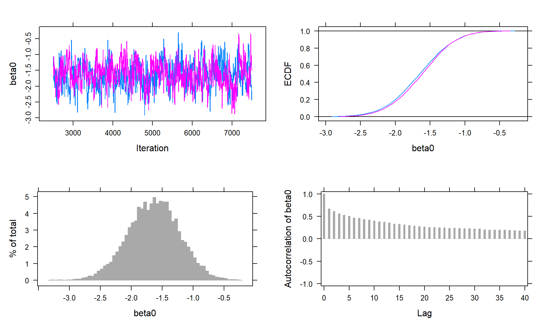
plot(jagsLogit, vars = "betaTrt")## Generating plots...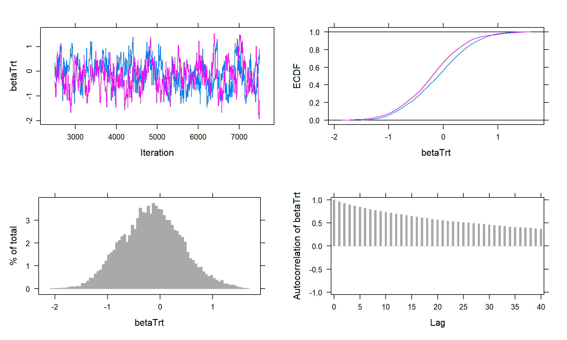

plot(jagsLogit, vars = "betaTime")## Generating plots...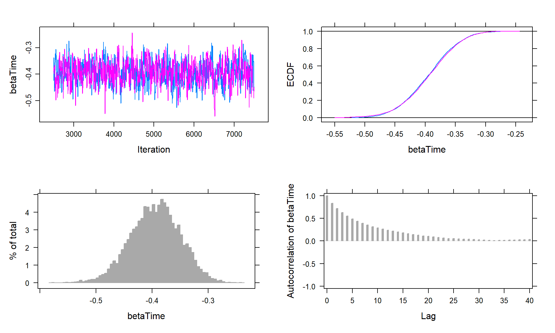
plot(jagsLogit, vars = "betaTrtTime")## Generating plots...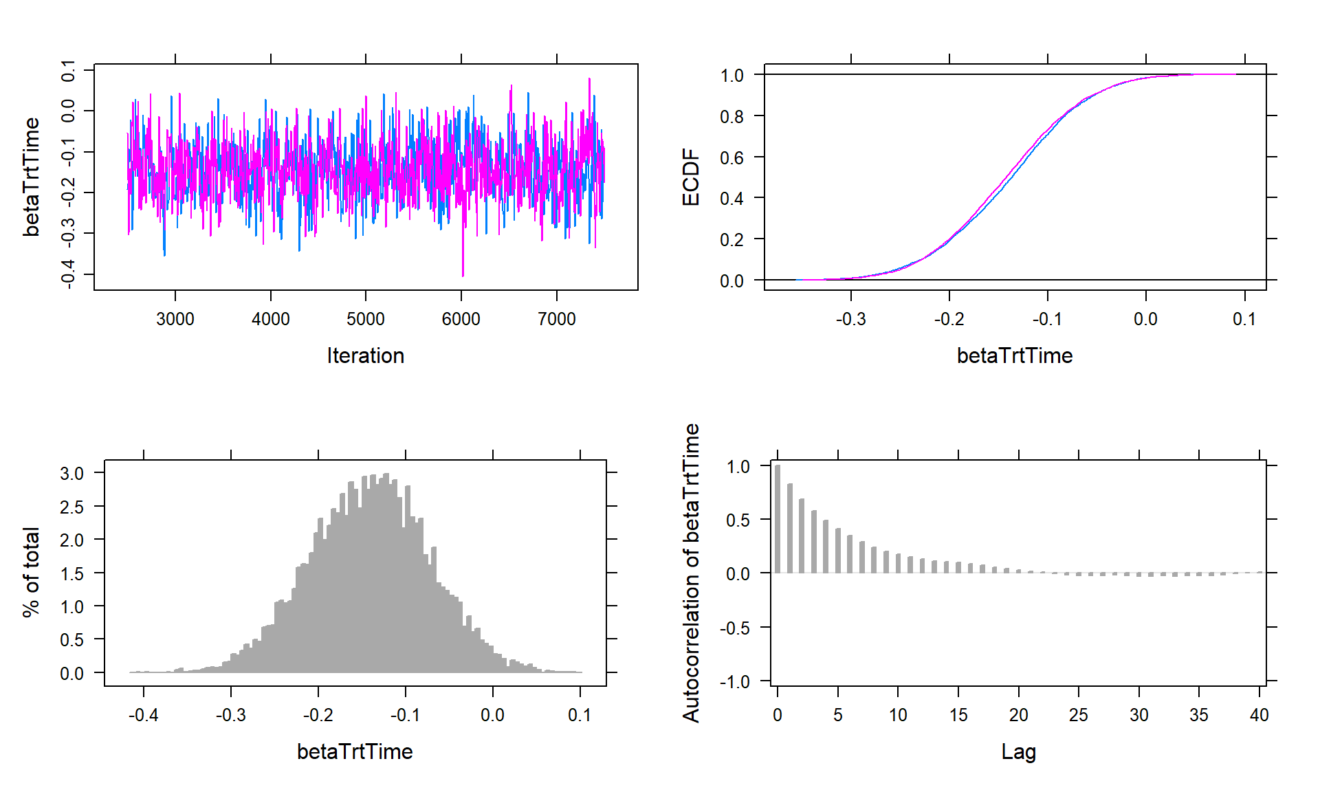
plot(jagsLogit, vars = "d0")## Generating plots...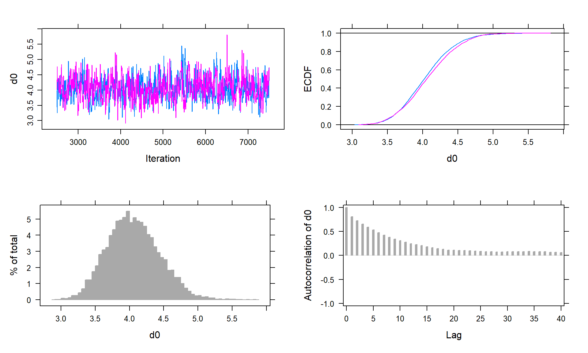
plot(jagsLogit, vars = "deviance")## Generating plots...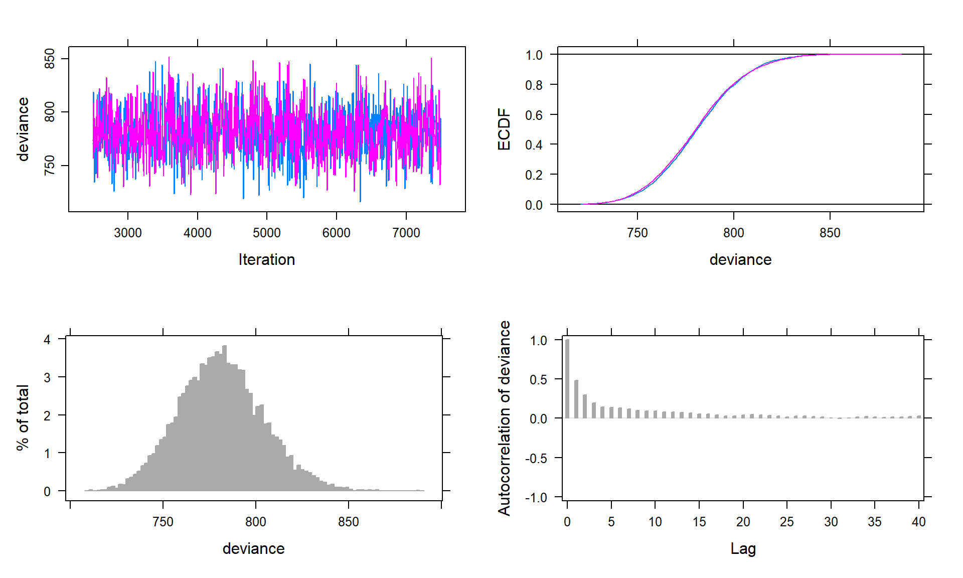
Only traceplots for selected parameters
Parm <- c("beta0", "betaTrt", "betaTime", "betaTrtTime", "d0", "deviance")
plot(jagsLogit, vars = Parm, plot.type = "trace", layout = c(2, 3))
## Generating plots...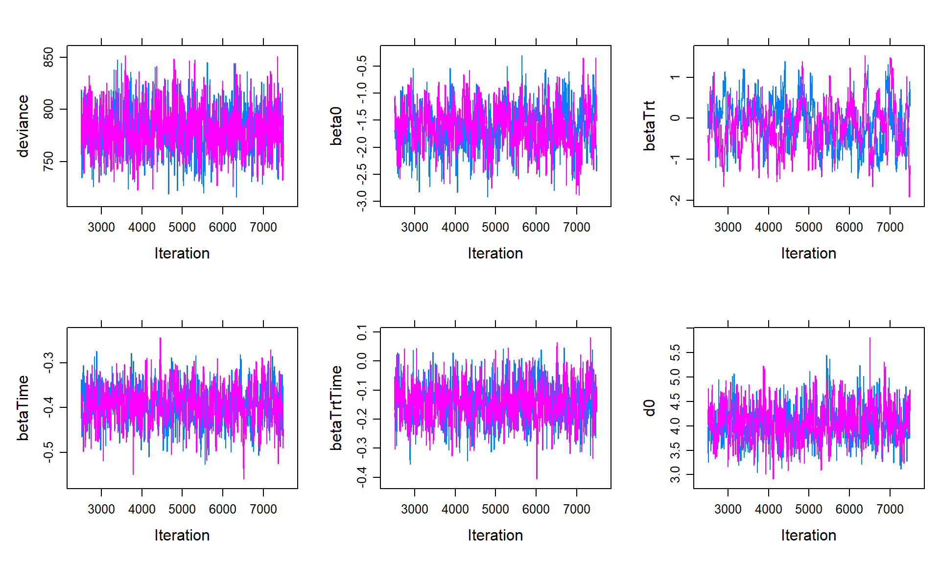
Only ECDF for selected parameters
plot(jagsLogit, vars = Parm, plot.type = "ecdf", layout = c(2, 3))## Generating plots...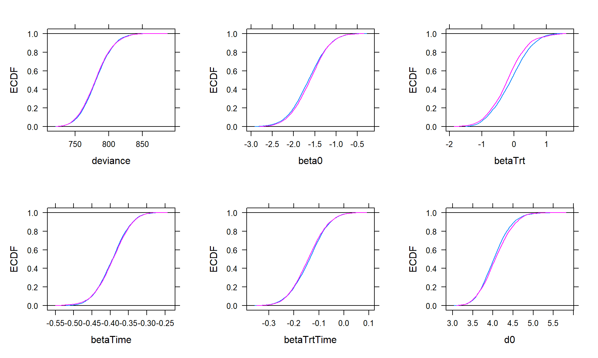
Only histograms for selected parameters
plot(jagsLogit, vars = Parm, plot.type = "histogram", layout = c(2, 3))## Generating plots...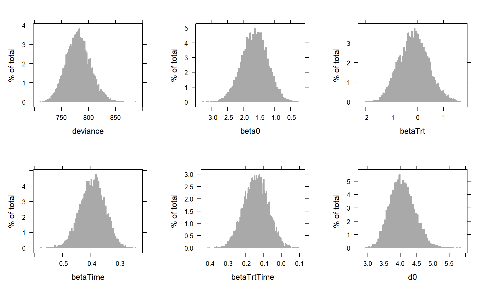
Only autocorrelation function (ACF) for selected parameters
plot(jagsLogit, vars = Parm, plot.type = "autocorr", layout = c(2, 3))## Generating plots...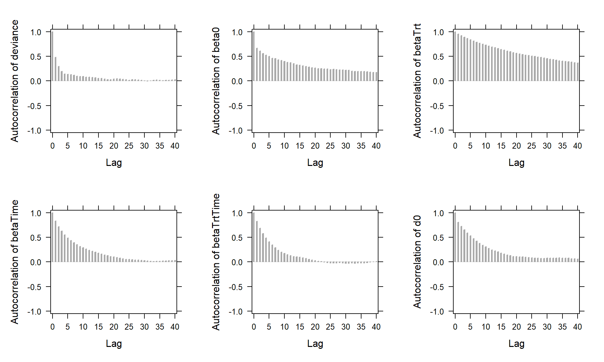
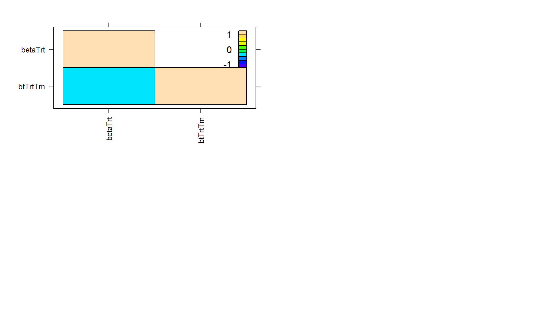
Crosscorrelations between chains of different parameters
plot(jagsLogit, plot.type = "crosscorr")## Generating plots...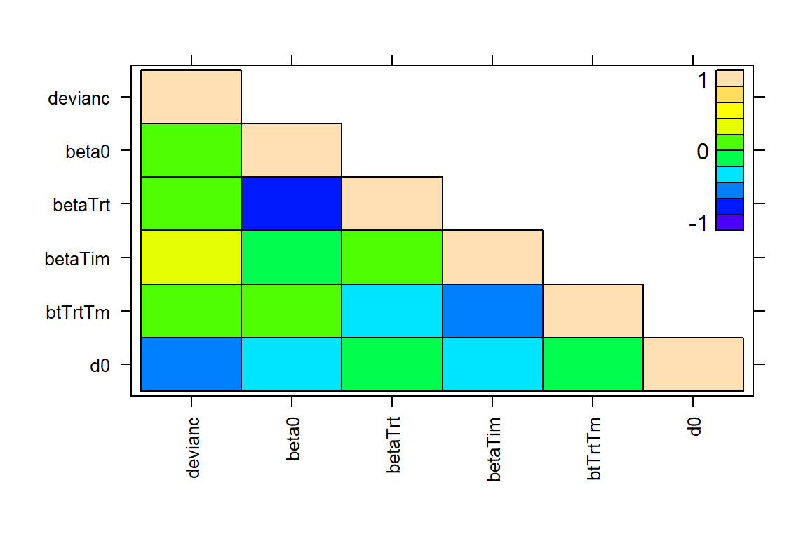
Gelman-Rubin convergence diagnostic
gelman.diag(jagsLogit$mcmc) # see help(coda::gelman.diag) for details## Potential scale reduction factors:
##
## Point est. Upper C.I.
## deviance 1 1.00
## beta0 1 1.00
## betaTrt 1 1.00
## betaTime 1 1.01
## betaTrtTime 1 1.00
## d0 1 1.00
##
## Multivariate psrf
##
## 1Geweke’s diagnostic (for beta’s only, separate set of plots for each chain)
geweke.diag(jagsLogit$mcmc) # see help(coda::geweke.diag) for details## [[1]]
##
## Fraction in 1st window = 0.1
## Fraction in 2nd window = 0.5
##
## deviance beta0 betaTrt betaTime betaTrtTime d0
## 1.3936 -2.3545 2.2850 1.8062 -0.2839 -1.8003
##
##
## [[2]]
##
## Fraction in 1st window = 0.1
## Fraction in 2nd window = 0.5
##
## deviance beta0 betaTrt betaTime betaTrtTime d0
## -0.3597 0.8957 -0.9319 -0.4243 0.1041 0.8677par(mfrow = c(2, 3))
geweke.plot(jagsLogit$mcmc[[1]]) # see help(coda::geweke.plot) for details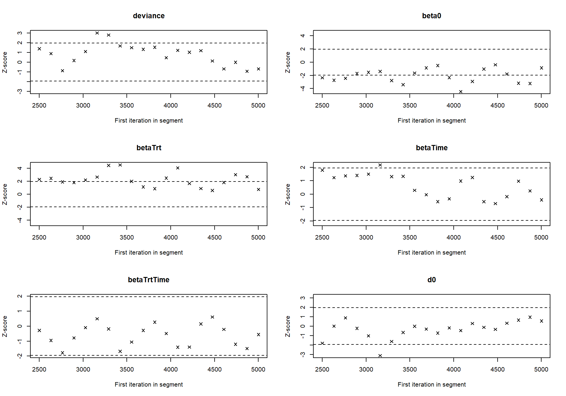
geweke.plot(jagsLogit$mcmc[[2]]) 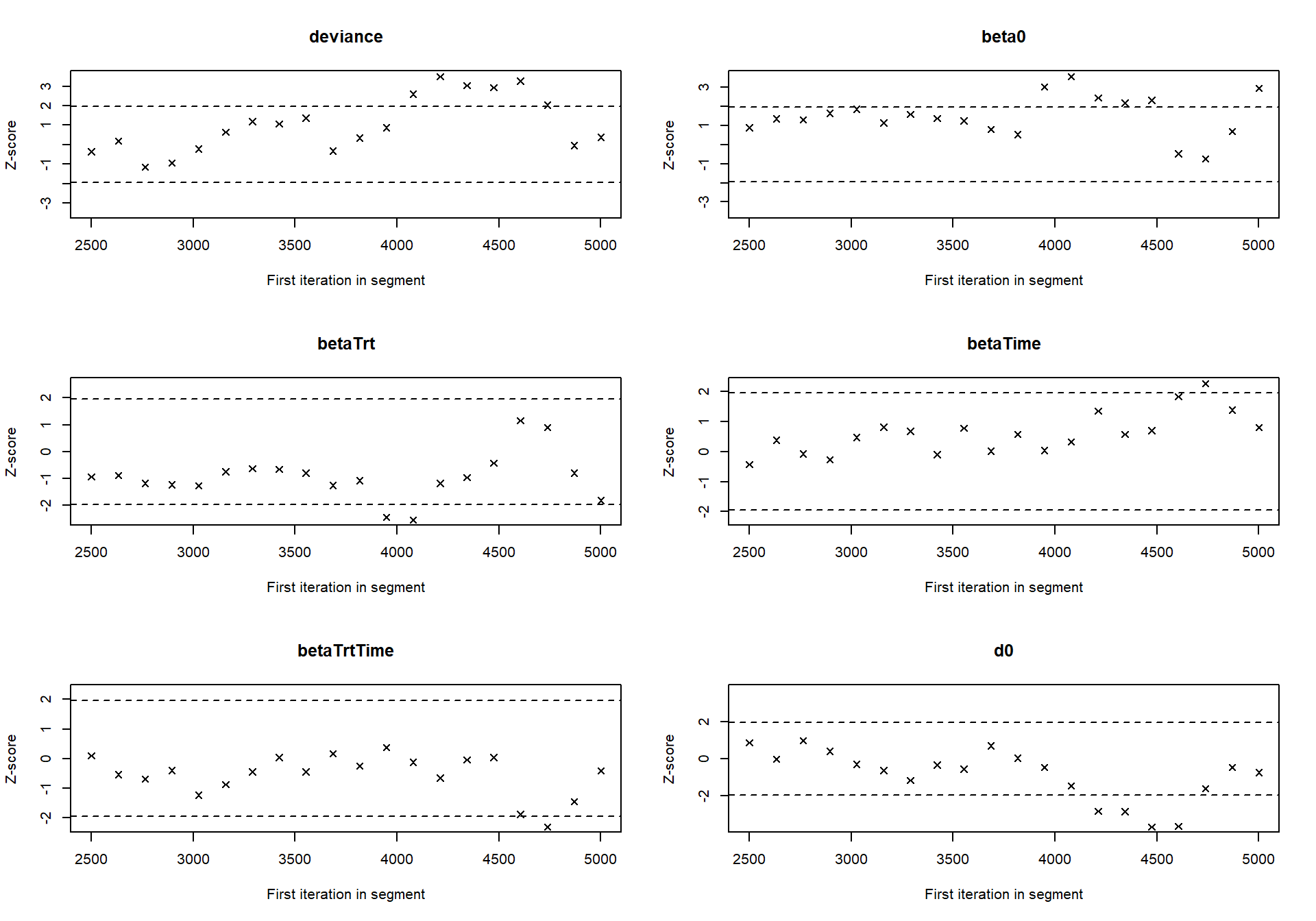
Task 4 - Exploring the posterior using MCMC samples
Let us now focus more on the estimates for regression coefficients. The basic summary is found here:
jagsLogit$summary##
## Iterations = 2501:7500
## Thinning interval = 1
## Number of chains = 2
## Sample size per chain = 5000
##
## 1. Empirical mean and standard deviation for each variable,
## plus standard error of the mean:
##
## Mean SD Naive SE Time-series SE
## deviance 781.1640 22.60763 0.2260763 0.538637
## beta0 -1.6362 0.41146 0.0041146 0.024327
## betaTrt -0.1539 0.56692 0.0056692 0.047059
## betaTime -0.3942 0.04426 0.0004426 0.001707
## betaTrtTime -0.1412 0.06814 0.0006814 0.002255
## d0 4.0583 0.38115 0.0038115 0.015467
##
## 2. Quantiles for each variable:
##
## 2.5% 25% 50% 75% 97.5%
## deviance 738.5098 765.4740 780.5268 795.66683 828.083173
## beta0 -2.4593 -1.9104 -1.6281 -1.35847 -0.843831
## betaTrt -1.2309 -0.5413 -0.1507 0.22448 0.996555
## betaTime -0.4821 -0.4239 -0.3930 -0.36394 -0.310694
## betaTrtTime -0.2757 -0.1878 -0.1398 -0.09485 -0.009839
## d0 3.3733 3.7911 4.0406 4.30634 4.829620The posterior SD for beta coefficients could be
extracted the following way:
beta_names <- rownames(jagsLogit$summary$statistics)[grep("^beta", rownames(jagsLogit$summary$statistics))]
(beta_post_sd <- jagsLogit$summary$statistics[beta_names, "SD"])
## beta0 betaTrt betaTime betaTrtTime
## 0.41146012 0.56692348 0.04426254 0.0681427610 / beta_post_sd # How many times the prior SD is larger than the posterior## beta0 betaTrt betaTime betaTrtTime
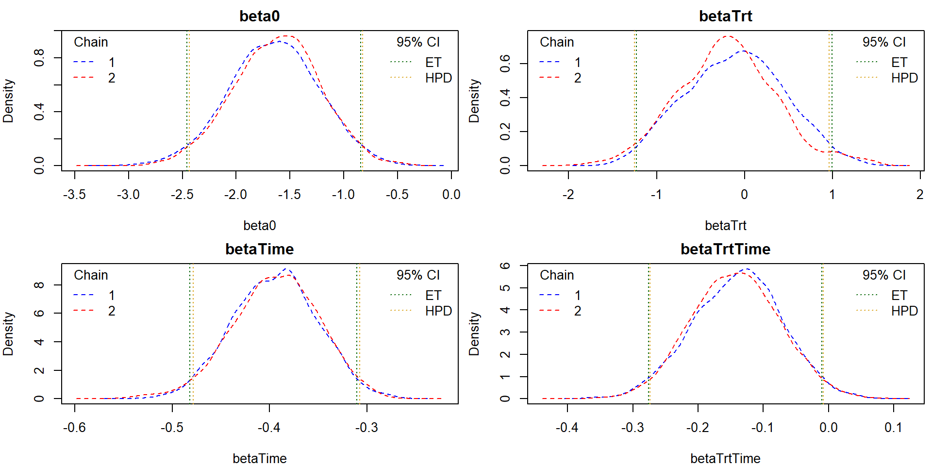
## 24.30369 17.63906 225.92470 146.75074We clearly see that the prior distribution has much larger variability and, thus, could be considered weakly informative (prior does not determine the results).
The credible intervals included within the summary are actually
Equal-Tailed (ET) credible intervals. These are constructed simply by
applying quantile with probabilities \(\frac{\alpha}{2}\) and \(1-\frac{\alpha}{2}\) to the relevant
samples. Compare for yourself:
(betaET <- jagsLogit$summary$quantiles[beta_names, paste0(c(2.5, 97.5),"%")])## 2.5% 97.5%
## beta0 -2.4593319 -0.843830911
## betaTrt -1.2308759 0.996554534
## betaTime -0.4820826 -0.310694291
## betaTrtTime -0.2756934 -0.009839341apply(jagsLogit$mcmc[[1]][, beta_names], 2, quantile, prob = c(0.025, 0.975)) # based only on chain 1## beta0 betaTrt betaTime betaTrtTime
## 2.5% -2.4887726 -1.1691506 -0.4780912 -0.27801656
## 97.5% -0.8405015 0.9597799 -0.3117766 -0.01105223beta_ET_manual <- t(apply(rbind(jagsLogit$mcmc[[1]][, beta_names],
jagsLogit$mcmc[[2]][, beta_names]),
2, quantile, prob = c(0.025, 0.975)))
all.equal(betaET, beta_ET_manual) # all values are equal up to a tolerance of cca 1e-8## [1] TRUEHighest Posterior Density (HPD) credible intervals are already calculated and available in the output.
print(jagsLogit$hpd)## Lower95 Median Upper95
## deviance 736.4761904 780.5267959 825.634046602
## beta0 -2.4367751 -1.6281094 -0.824945182
## betaTrt -1.2541763 -0.1507082 0.962809401
## betaTime -0.4784368 -0.3930500 -0.307685839
## betaTrtTime -0.2734764 -0.1398445 -0.008082525
## d0 3.3567881 4.0406127 4.798241556print(jagsLogit$HPD) # the same## Lower95 Median Upper95
## deviance 736.4761904 780.5267959 825.634046602
## beta0 -2.4367751 -1.6281094 -0.824945182
## betaTrt -1.2541763 -0.1507082 0.962809401
## betaTime -0.4784368 -0.3930500 -0.307685839
## betaTrtTime -0.2734764 -0.1398445 -0.008082525
## d0 3.3567881 4.0406127 4.798241556HPDinterval(jagsLogit$mcmc) # computation for each chain separately## [[1]]
## lower upper
## deviance 740.4243142 828.57241707
## beta0 -2.4761178 -0.83466025
## betaTrt -1.1359195 0.99060590
## betaTime -0.4785272 -0.31269622
## betaTrtTime -0.2723474 -0.00574563
## d0 3.3184719 4.75738304
## attr(,"Probability")
## [1] 0.95
##
## [[2]]
## lower upper
## deviance 736.4761904 826.44550290
## beta0 -2.3986704 -0.81483877
## betaTrt -1.4763780 0.84495823
## betaTime -0.4828919 -0.30815141
## betaTrtTime -0.2745482 -0.01097416
## d0 3.3571517 4.79796072
## attr(,"Probability")
## [1] 0.95See help(coda::HPDinterval) for some details. For each
parameter the interval is constructed from the ECDF of the
sample as the shortest interval for which the
difference in the ECDF values of the endpoints is the nominal
probability. Assuming that the distribution is not
severely multimodal, this is the HPD interval.
When the samples are cleared of high autocorrelation (higher
thin), basically any approach for approximation of a
characteristic of a distribution can be used to approximate the same
characteristic of posterior distribution. For example, let us use kernel
density estimators for the coefficients:
COL <- c("blue", "red")
par(mfrow = c(2,2), mar = c(4,4,2,0.5))
for(beta in beta_names){
  dens <- lapply(jagsLogit$mcmc, function(mcmc){density(mcmc[,beta])})
  rangex <- range(unlist(lapply(dens, function(d){range(d$x)})))
  rangey <- range(unlist(lapply(dens, function(d){range(d$y)})))

  plot(0,0,type = "n", xlim = rangex, ylim = rangey,
       xlab = beta, ylab = "Density", main = beta)
  for(i in 1:length(dens)){
    lines(dens[[i]], col = COL[i], lty = 2)
    abline(v = jagsLogit$summary$quantiles[beta,c("2.5%", "97.5%")], col = "darkgreen", lty = 3)
    abline(v = jagsLogit$HPD[beta, c("Lower95", "Upper95")], col = "goldenrod", lty = 3)
  }
  legend("topleft", legend = 1:length(dens), title = "Chain", col = COL, lty = 2, bty = "n")
  legend("topright", c("ET", "HPD"), title = "95% CI", col = c("darkgreen", "goldenrod"), lty = 3, bty = "n")
}
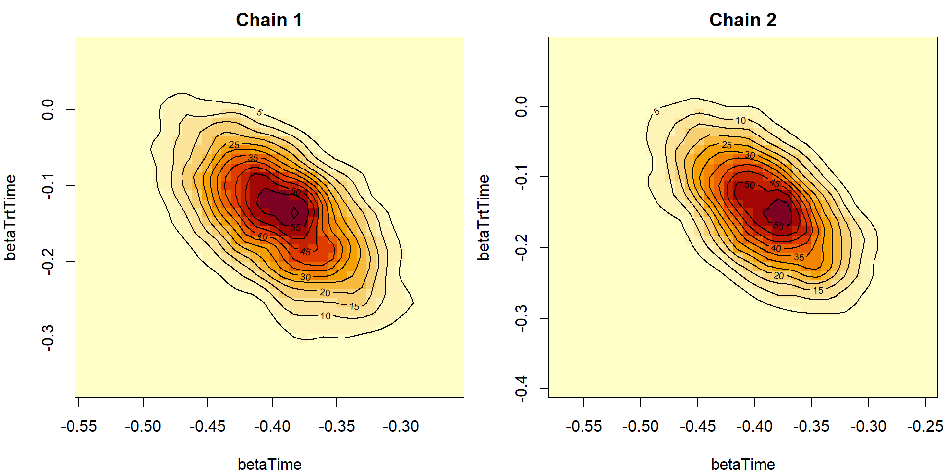
Or even a bivariate version including the contours:
library(MASS)
# ?MASS::kde2d
dens <- lapply(jagsLogit$mcmc, function(mcmc){kde2d(x = mcmc[,"betaTime"],
                                                    y = mcmc[,"betaTrtTime"],
                                                    n = 40)})
# rangex <- range(unlist(lapply(dens, function(d){range(d$x)})))
# rangey <- range(unlist(lapply(dens, function(d){range(d$y)})))
rangez <- range(unlist(lapply(dens, function(d){range(d$z)})))

par(mfrow = c(1,2), mar = c(4,4,2,0.5))
for(ch in 1:length(dens)){
  image(dens[[ch]],
        zlim = rangez, # xlim = rangex, ylim = rangey,
        main = paste("Chain", ch), xlab = "betaTime", ylab = "betaTrtTime")
  contour(dens[[ch]], add = T)
}
Task 5+6 - Additional parameters of interest
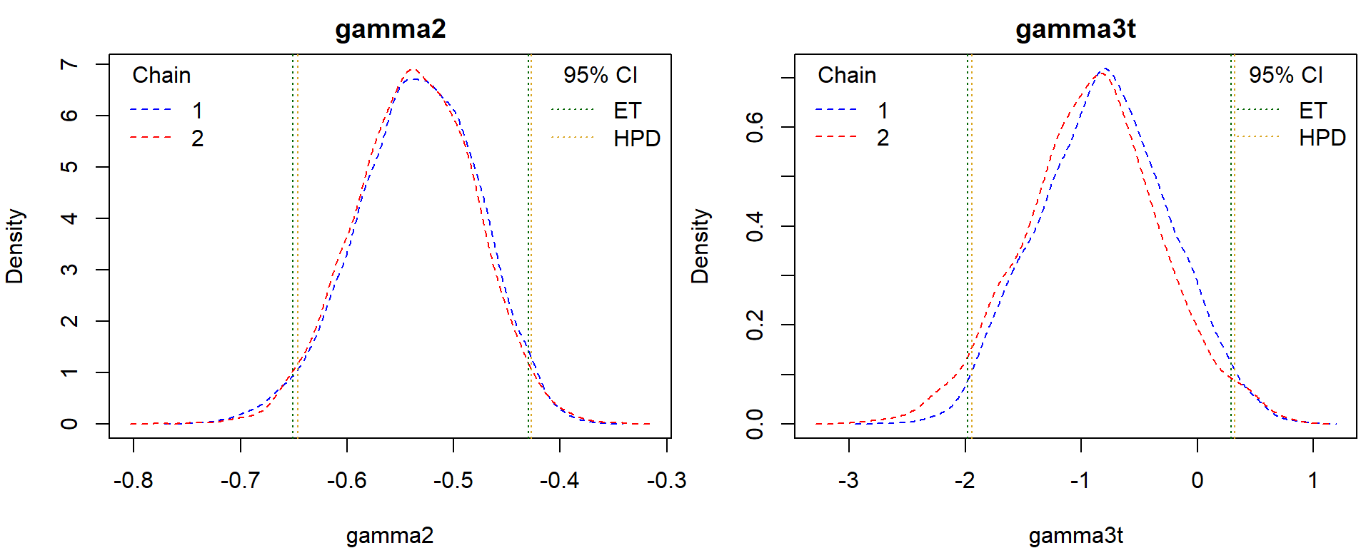
When we read carefully the assignment, we decode that * \(d_0 = \tau_0^{-1/2}\) = d0,. *
\(\gamma_1 = \beta_2\) =
betaTime, * \(\gamma_2 =
\beta_2+\beta_3\) = betaTime + betaTrtTime, * \(\gamma_3(t) = \beta_1+ t \beta_3\) =
betaTime + t * betaTrtTime, (B compared to A), which
depends on the time t.
First two parameters are already included within out sampled states.
The posterior summary is already at our disposal within
jagsLogit object.
summary(jagsLogit, vars = c("d0", "betaTime"))## Lower95 Median Upper95 Mean SD Mode MCerr MC%ofSD SSeff AC.10 psrf
## d0 3.3567881 4.040613 4.7982416 4.0582529 0.38115280 NA 0.015472730 4.1 607 0.3067187 1.002775
## betaTime -0.4784368 -0.393050 -0.3076858 -0.3941664 0.04426254 NA 0.001703483 3.8 675 0.2900291 1.000650The posterior density estimate + credible intervals (based on both chains):
COL <- c("blue", "red")
par(mfrow = c(1,2), mar = c(4,4,2,0.5))
for(var in c("d0", "betaTime")){
dens <- lapply(jagsLogit$mcmc, function(mcmc){density(mcmc[,var])})
rangex <- range(unlist(lapply(dens, function(d){range(d$x)})))
rangey <- range(unlist(lapply(dens, function(d){range(d$y)})))
plot(0,0,type = "n", xlim = rangex, ylim = rangey,
xlab = var, ylab = "Density", main = var)
for(i in 1:length(dens)){
lines(dens[[i]], col = COL[i], lty = 2)
abline(v = jagsLogit$summary$quantiles[var,c("2.5%", "97.5%")], col = "darkgreen", lty = 3)
abline(v = jagsLogit$HPD[var,c("Lower95", "Upper95")], col = "goldenrod", lty = 3)
}
legend("topleft", legend = 1:length(dens), title = "Chain", col = COL, lty = 2, bty = "n")
legend("topright", c("ET", "HPD"), title = "95% CI", col = c("darkgreen", "goldenrod"), lty = 3, bty = "n")
}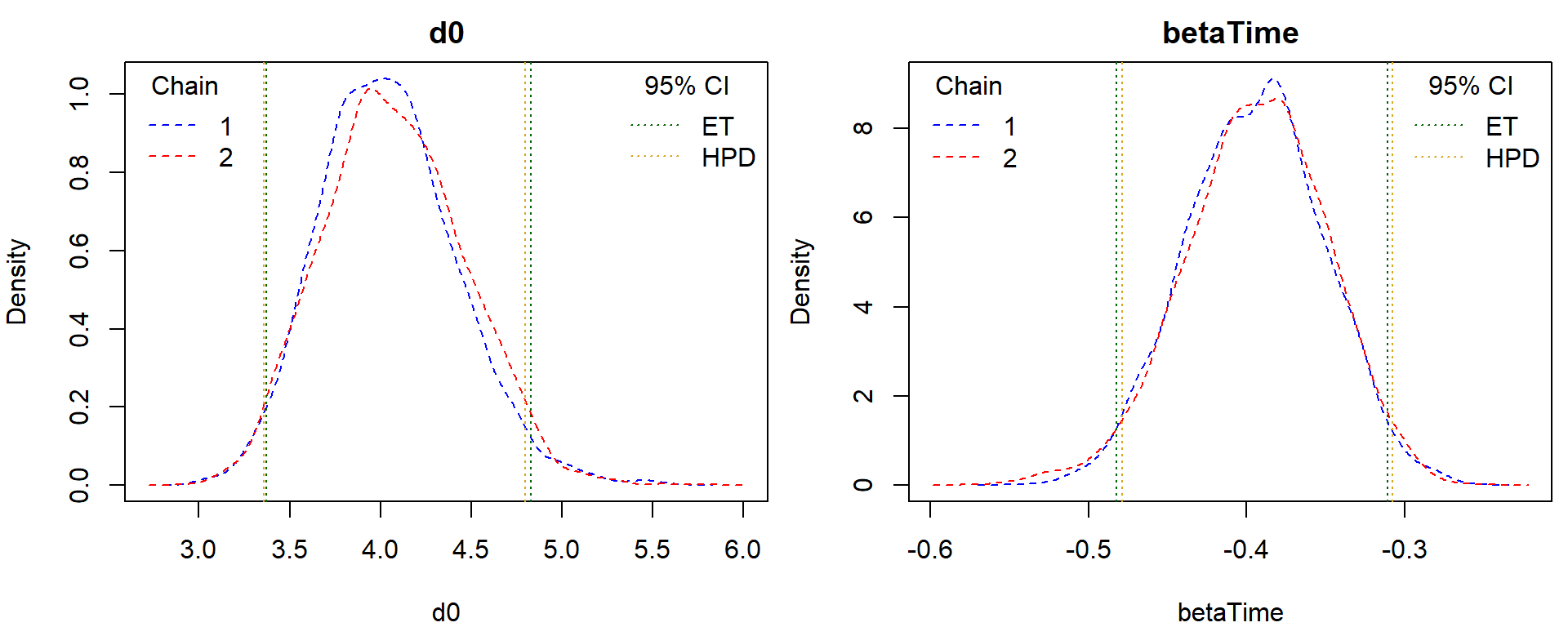 The other parameters are not included among the monitored parameters
(unless time
The other parameters are not included among the monitored parameters
(unless time t=0). One way to obtain all necessary
estimates would be to include them in the Model definition,
the same way as d0 was. But we would have to run the
sampling algorithm once again, which is time and energy consuming.
However, we already have the samples at our disposal. The quantities of interest are actually a simple transformation of the other available parameters. Their samples are then corresponding deterministic transformation of the available samples.
t <- 5                 # chosen value for time
my_mcmc <- list()
for(ch in 1:2){
  my_mcmc[[ch]] <- data.frame(jagsLogit$mcmc[[ch]][,"betaTime"] + jagsLogit$mcmc[[ch]][,"betaTrtTime"],
                              jagsLogit$mcmc[[ch]][,"betaTrt"] + t * jagsLogit$mcmc[[ch]][,"betaTrtTime"])
  colnames(my_mcmc[[ch]]) <- c("gamma2", "gamma3t")
  start_end <- attr(jagsLogit$mcmc[[ch]], "mcpar")
  my_mcmc[[ch]] <- mcmc(my_mcmc[[ch]],         # creating my own class(mcmc)
                        start = start_end[1],  # jagsLogit$burnin + 1
                        end = start_end[2],    # jagsLogit$burnin + jagsLogit$sample
                        thin = jagsLogit$thin) # start_end[3]
}
class(my_mcmc)
## [1] "list"my_mcmc <- as.mcmc.list(my_mcmc) # now of class mcmc.list
(sum_my_mcmc <- summary(my_mcmc)) # uses corresponding summary method for class mcmc.list##
## Iterations = 2501:7500
## Thinning interval = 1
## Number of chains = 2
## Sample size per chain = 5000
##
## 1. Empirical mean and standard deviation for each variable,
## plus standard error of the mean:
##
## Mean SD Naive SE Time-series SE
## gamma2 -0.5353 0.05657 0.0005657 0.001515
## gamma3t -0.8597 0.58167 0.0058167 0.036654
##
## 2. Quantiles for each variable:
##
## 2.5% 25% 50% 75% 97.5%
## gamma2 -0.651 -0.5731 -0.5341 -0.4951 -0.4299
## gamma3t -1.980 -1.2471 -0.8509 -0.4710 0.2893With the new mcmc.list object we can use all methods as
directly for any mcmc object.
par(mfrow = c(1,2), mar = c(4,4,2,0.5))
plot(my_mcmc, trace = TRUE, density = FALSE)![]()
It remains to compute HPD credible intervals (ET already within the summary).
# chains separately
HPDinterval(my_mcmc)
## [[1]]
## lower upper
## gamma2 -0.6405184 -0.4225237
## gamma3t -1.9131283 0.2307188
## attr(,"Probability")
## [1] 0.95
##
## [[2]]
## lower upper
## gamma2 -0.6476215 -0.4296092
## gamma3t -2.0836491 0.3114352
## attr(,"Probability")
## [1] 0.95# both chains together
(gammaHPD <- HPDinterval(as.mcmc(rbind(my_mcmc[[1]], my_mcmc[[2]]))))## lower upper
## gamma2 -0.6459985 -0.4270590
## gamma3t -1.9448524 0.3201626
## attr(,"Probability")
## [1] 0.95COL <- c("blue", "red")
par(mfrow = c(1,2), mar = c(4,4,2,0.5))
for(var in c("gamma2", "gamma3t")){
dens <- lapply(my_mcmc, function(mcmc){density(mcmc[,var])})
rangex <- range(unlist(lapply(dens, function(d){range(d$x)})))
rangey <- range(unlist(lapply(dens, function(d){range(d$y)})))
plot(0,0,type = "n", xlim = rangex, ylim = rangey,
xlab = var, ylab = "Density", main = var)
for(i in 1:length(dens)){
lines(dens[[i]], col = COL[i], lty = 2)
abline(v = sum_my_mcmc$quantiles[var,c("2.5%", "97.5%")], col = "darkgreen", lty = 3)
abline(v = gammaHPD[var,c("lower", "upper")], col = "goldenrod", lty = 3)
}
legend("topleft", legend = 1:length(dens), title = "Chain", col = COL, lty = 2, bty = "n")
legend("topright", c("ET", "HPD"), title = "95% CI", col = c("darkgreen", "goldenrod"), lty = 3, bty = "n")
}
Once we have samples of model parameters, exploring the posterior of some parametric function is only a matter of transformation. Other potential parametric functions of interest:
- exponential transformations of the coefficients,
- odds ratios for comparing two patients of the same predisposition for infection (measured by random intercept),
- probability of infection with certain drug and at certain time under optimistic, realistic or pesimistic scenario,
- possibly even for a grid of time values, not just one.
Task 7 - Probability resembling p-value
The goal is to find the lowest coverage for ET intervals such that 0 is not contained within the ET interval. We will showcase this on \(\gamma_3(t)\).
Lets start slowly by finding the posterior median:
(gamma3t_med <- sum_my_mcmc$quantiles["gamma3t", "50%"])## [1] -0.8508945(which_side <- ifelse(gamma3t_med < 0, "upper", "lower"))## [1] "upper"Now we know which end of the interval (lower or upper) will touch 0. Let us formulate the function that measures how far is the upper bound from zero.
# First, for simplicity, take all samples of the parameter into one vector
gamma3t <- c(my_mcmc[[1]][,"gamma3t"], my_mcmc[[2]][,"gamma3t"])

dist_ET_from_0 <- function(alpha){
  quantile(gamma3t, prob = 1-alpha/2) - 0 # not a distance (also negative values)
}
The Bayesian version of p-value is now root of the defined function:
gamma3t_pvalue <- uniroot(dist_ET_from_0, interval = c(0, 1))
gamma3t_pvalue$root
## [1] 0.1415897# check, whether it truly satisfies the property
quantile(gamma3t, probs = c(gamma3t_pvalue$root/2, 1-gamma3t_pvalue$root/2))## 7.079485% 92.92052%
## -1.731470e+00 1.674243e-05Let me summarize the process into a function:
bayes_pvalue <- function(x, x0 = 0){
  medx <- median(x)
  rangex <- range(x)
  if((rangex[1]-x0) * (rangex[2]-x0) > 0){    # same signs (all sampled values on the same side from x0)
    return(0)                                 # we are pretty sure, parameter x is far away from x0
  }else{                                      # opposite signs (x0 between sampled values)
    if(medx < x0){
      dist_ET_from_x0 <- function(alpha){
        quantile(x, prob = 1-alpha/2) - x0
      }
    }else{
      dist_ET_from_x0 <- function(alpha){
        quantile(x, prob = alpha/2) - x0
      }
    }
    root <- uniroot(dist_ET_from_x0, interval = c(0, 1))
    return(root$root)
  }
}
Lets check whether it works (one both chains):
# betaTrt
jagsLogit$summary$quantiles["betaTrt",]
## 2.5% 25% 50% 75% 97.5%
## -1.2308759 -0.5413178 -0.1507082 0.2244847 0.9965545bayes_pvalue(c(jagsLogit$mcmc[[1]][,"betaTrt"], jagsLogit$mcmc[[2]][,"betaTrt"]))## [1] 0.7824862# betaTime
jagsLogit$summary$quantiles["betaTime",]## 2.5% 25% 50% 75% 97.5%
## -0.4820826 -0.4238685 -0.3930500 -0.3639371 -0.3106943bayes_pvalue(c(jagsLogit$mcmc[[1]][,"betaTime"], jagsLogit$mcmc[[2]][,"betaTime"]))## [1] 0bayes_pvalue(c(jagsLogit$mcmc[[1]][,"betaTime"], jagsLogit$mcmc[[2]][,"betaTime"]), -0.3)## [1] 0.02415119# betaTrtTime
jagsLogit$summary$quantiles["betaTrtTime",]## 2.5% 25% 50% 75% 97.5%
## -0.275693376 -0.187831784 -0.139844469 -0.094849163 -0.009839341bayes_pvalue(c(jagsLogit$mcmc[[1]][,"betaTrtTime"], jagsLogit$mcmc[[2]][,"betaTrtTime"]))## [1] 0.03424467