Non-parametric estimation of cumulative hazard and survival function
Jan Vávra
Exercise 2
Lecture revision: non-parametric estimation, confidence intervals and bands
Theory
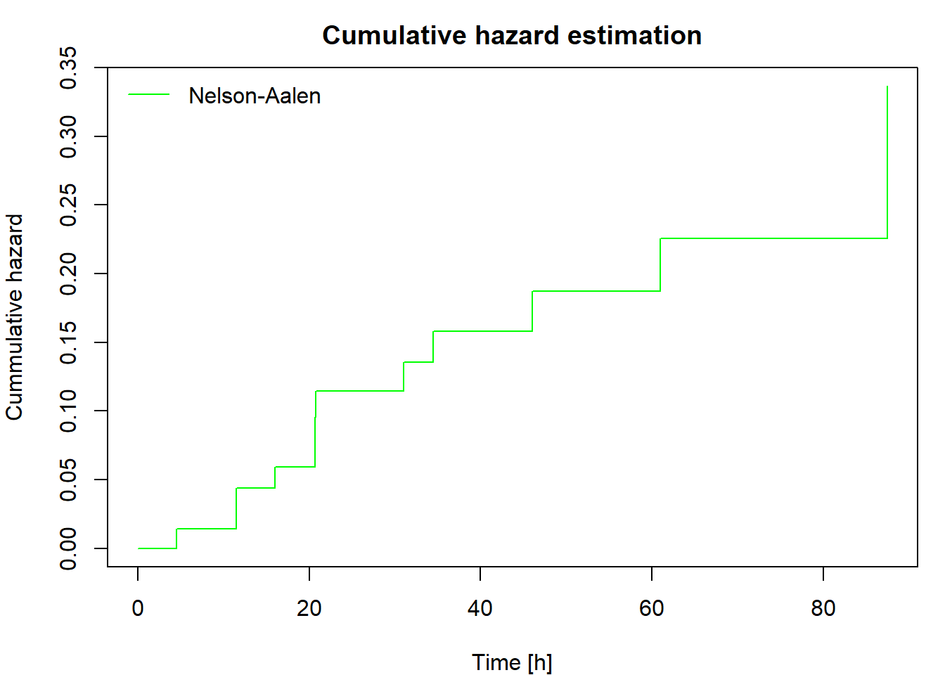
The cumulative hazard can be estimated non-parametrically by the Nelson-Aalen estimator defined as
\[ \widehat{\Lambda}(t)=\int_0^t\frac{\,\mathrm{d} \overline{N}(u)}{\overline{Y}(u)}= \sum_{\{i: t_i\leq t\}} \frac{\Delta\overline{N}(t_i)}{\overline{Y}(t_i)}, \] where \(0<t_1<t_2<\cdots<t_d\) are ordered distinct failure times.
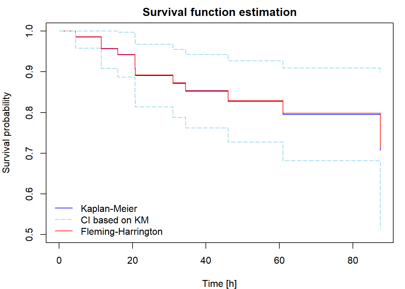
The Kaplan-Meier [KM] estimator of the survival function is \[ \widehat{S}(t) = \prod_{\{i: t_i\leq t\}}\biggl[1-\frac{\Delta\overline{N}(t_i)}{\overline{Y}(t_i)}\biggr] = \widehat{S}(t-) \cdot \biggl[1-\frac{\Delta\overline{N}(t)}{\overline{Y}(t)}\biggr]. \] A uniformly consistent estimator of the variance of \(\sqrt{n}[\widehat{S}(t)-S(t)]\) is (by Greenwood formula) \[ \widehat{V}(t) = \widehat{S}^2(t)\widehat{\sigma}(t) = \widehat{S}^2(t)\int_0^t \frac{n \,\mathrm{d}\overline{N}(u)}{\overline{Y}(u)[\overline{Y}(u)-\Delta\overline{N}(u)]} = \widehat{S}^2(t) \cdot n \cdot \sum \limits_{\{i:t_i \leq t\}} \dfrac{\Delta \overline{N}(t_i)}{\overline{Y}(t_i)[\overline{Y}(t_i)-\Delta\overline{N}(t_i)]}. \] We use this estimator for construction of asymptotic confidence intervals. An asymptotic pointwise \(100(1-\alpha)\)% confidence interval for \(S(t)\) at a fixed \(t\) is \[ \biggl( \widehat{S}(t)\Bigl[1-u_{1-\alpha/2}\sqrt{\widehat{\sigma}(t)/n}\Bigr],\, \widehat{S}(t)\Bigl[1+u_{1-\alpha/2}\sqrt{\widehat{\sigma}(t)/n}\Bigr] \biggr). \]
If the distribution of \(T_i\) is continuous, one could define an alternative survival function estimator using the relationship \(S(t)=\exp\{-\Lambda(t)\}\) applied to the Nelson-Aalen estimator, that is \[ \widehat{S}_*(t)=\exp\{-\widehat{\Lambda}(t)\}=\prod_{\{i: t_i\leq t\}}\exp\biggl\{-\frac{\Delta\overline{N}(t_i)}{\overline{Y}(t_i)}\biggr\}. \] This is called the Fleming-Harrington [FH] estimator (sometimes also the Breslow estimator). Because \(\exp\{-h\}\approx 1-h\) for small \(h\), the difference between the KM and FH estimators is small unless the risk set size \(\overline{Y}(u)\) is not large enough, which happens at the largest failure times. The FH estimator is not suitable for discrete data, while the KM estimator works well for both discrete and continuous cases.
Understanding the formulae
The dataset fans [Nelson, Journal of Quality Technology,
1:27-52, 1969] comes from an engineering study of the time to failure of
diesel generator fans. Seventy generators were studied. For each one,
the number of hours of running time from its first being put into
service until fan failure or until the end of the study (whichever came
first) was recorded.
The data is available in the RData format from this link.
The dataframe is called fans, the variable
fans$time includes the censored failure time \(X_i\) (in hours), the variable
fans$fail is the failure indicator \(\delta_i\).
We will use this dataset to demonstrate the calculation of cumulative hazard and survival function estimates.
Using ordinary R functions (table, cumsum,
cumprod, rev, …, but not functions from the
survival library), calculate and print the following
table:
i |
time |
n.risk |
n.event |
cumhaz |
survivalKM |
survivalFH |
std.err |
l95CI |
u95CI |
|---|---|---|---|---|---|---|---|---|---|
| 1 | … | … | … | … | … | … | … | … | … |
| … | … | … | … | … | … | … | … | … | … |
| d | … | … | … | … | … | … | … | … | … |
where i is the order of the failures, time
is the ordered failure time (print only times with
n.event > 0), n.risk\(=\overline{Y}(t_i)\),
n.event\(=\Delta\overline{N}(t_i)\),
cumhaz\(=\widehat{\Lambda}(t_i)\),
survivalKM\(=\widehat{S}(t_i)\),
survivalFH\(=\widehat{S}_*(t_i)\)
std.err\(=\widehat{S}(t_i) \cdot
\sqrt{\widehat{\sigma}(t_i) / n}\), l95CI\(=\max\left\{0,
\widehat{S}(t)\Bigl[1-u_{0.975}\sqrt{\widehat{\sigma}(t)/n}\Bigr]\right\}\),
u95CI\(=\min\left\{1,
\widehat{S}(t)\Bigl[1+u_{0.975}\sqrt{\widehat{\sigma}(t)/n}\Bigr]\right\}\).
Then plot the cumulative hazard estimator and both survival function estimators. Include in your report the code for calculating and plotting the results and the output you obtained.
Calculating the estimators using library(survival)
The basic functions for censored data analysis are available in R
library survival. Censored data are entered as special
survival objects created in this way:
library(survival)
Surv(time, delta)
## see help(Surv)
# used as a response variable in a model formula
# right censoring is set as default
where time is a numeric vector containing the censored
failure times and delta is a numeric vector containing
failure indicators (1 = failure, 0 = censored). Survival objects are
used as input to functions providing analysis of censored data.
Survival function estimates are calculated by the function
survfit. The most rudimentary use of this function is
fit <- survfit(Surv(time, delta) ~ 1, data = data)This calculates the KM estimator. The FH estimator is obtained by
adding an option type or correct combination of
stype and ctype:
fit <- survfit(Surv(time, delta) ~ 1, type = "fleming", data = data)
fit <- survfit(Surv(time, delta) ~ 1, stype = 2, ctype = 1, data = data)
stype = 1- direct estimation of survival (Kaplan-Meier),stype = 2- survival function estimated byexp(-cumhaz)(Fleming-Harrington),ctype = 1- cumulative hazard estimated via Nelson-Aalen,ctype = 2- Fleming-Harrington correction for tied events in cumulative hazard estimator.
Combinations:
type = 'kaplan-meier'is equivalent tostype = 1, ctype = 1,type = 'fleming-harrington'is equivalent tostype = 2, ctype = 1,type = 'fh2'is equivalent tostype = 2, ctype = 2.
Notice, that the default option for the type of confidence intervals
is conf.int = "log", which applies Delta theorem with \(\log\) transformation to obtain slightly
different CI than the "plain" option described and computed
in Task 1.
The results can be plotted easily by calling
plot(fit)
?plot.survfit
For demonstration, we will use the dataset aml included
in library(survival). Survival in patients with Acute
Myelogenous Leukemia. The question at the time was whether the standard
course of chemotherapy should be extended (‘maintenance’) for additional
cycles.
print(aml)## time status x
## 1 9 1 Maintained
## 2 13 1 Maintained
## 3 13 0 Maintained
## 4 18 1 Maintained
## 5 23 1 Maintained
## 6 28 0 Maintained
## 7 31 1 Maintained
## 8 34 1 Maintained
## 9 45 0 Maintained
## 10 48 1 Maintained
## 11 161 0 Maintained
## 12 5 1 Nonmaintained
## 13 5 1 Nonmaintained
## 14 8 1 Nonmaintained
## 15 8 1 Nonmaintained
## 16 12 1 Nonmaintained
## 17 16 0 Nonmaintained
## 18 23 1 Nonmaintained
## 19 27 1 Nonmaintained
## 20 30 1 Nonmaintained
## 21 33 1 Nonmaintained
## 22 43 1 Nonmaintained
## 23 45 1 NonmaintainedWe get a full description of our estimates of survival function by
summary applied to survfit object:
fit_KM <- survfit(Surv(time, status) ~ 1, data = aml)
summary(fit_KM)
## Call: survfit(formula = Surv(time, status) ~ 1, data = aml)
##
## time n.risk n.event survival std.err lower 95% CI upper 95% CI
## 5 23 2 0.9130 0.0588 0.8049 1.000
## 8 21 2 0.8261 0.0790 0.6848 0.996
## 9 19 1 0.7826 0.0860 0.6310 0.971
## 12 18 1 0.7391 0.0916 0.5798 0.942
## 13 17 1 0.6957 0.0959 0.5309 0.912
## 18 14 1 0.6460 0.1011 0.4753 0.878
## 23 13 2 0.5466 0.1073 0.3721 0.803
## 27 11 1 0.4969 0.1084 0.3240 0.762
## 30 9 1 0.4417 0.1095 0.2717 0.718
## 31 8 1 0.3865 0.1089 0.2225 0.671
## 33 7 1 0.3313 0.1064 0.1765 0.622
## 34 6 1 0.2761 0.1020 0.1338 0.569
## 43 5 1 0.2208 0.0954 0.0947 0.515
## 45 4 1 0.1656 0.0860 0.0598 0.458
## 48 2 1 0.0828 0.0727 0.0148 0.462We calculate and plot KM and FH estimates like this
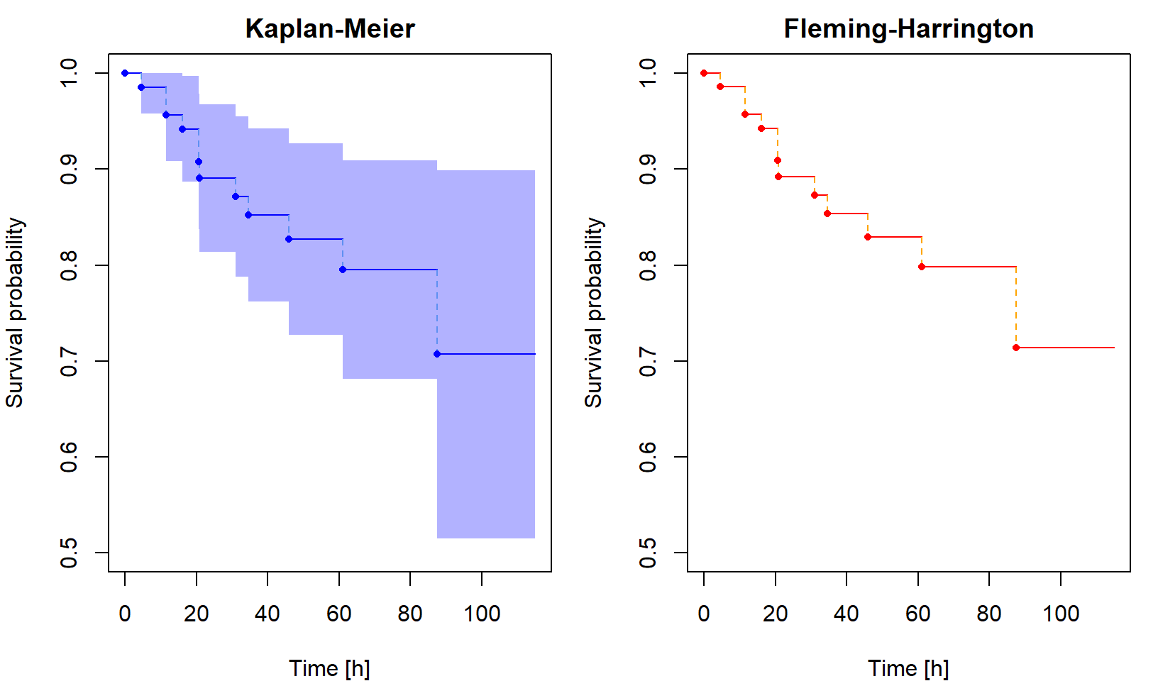
fit_FH <- survfit(Surv(time, status) ~ 1, type = "fleming", data = aml)

par(mar = c(4,4,1,1))
plot(fit_KM, xlab = "Time", ylab = "Survival probability", col = "blue")
lines(fit_FH, col = "red")
legend("topright", c("Kaplan-Meier", "Fleming-Harrington"),
       col = c("blue", "red"), lty = 1, bty = "n")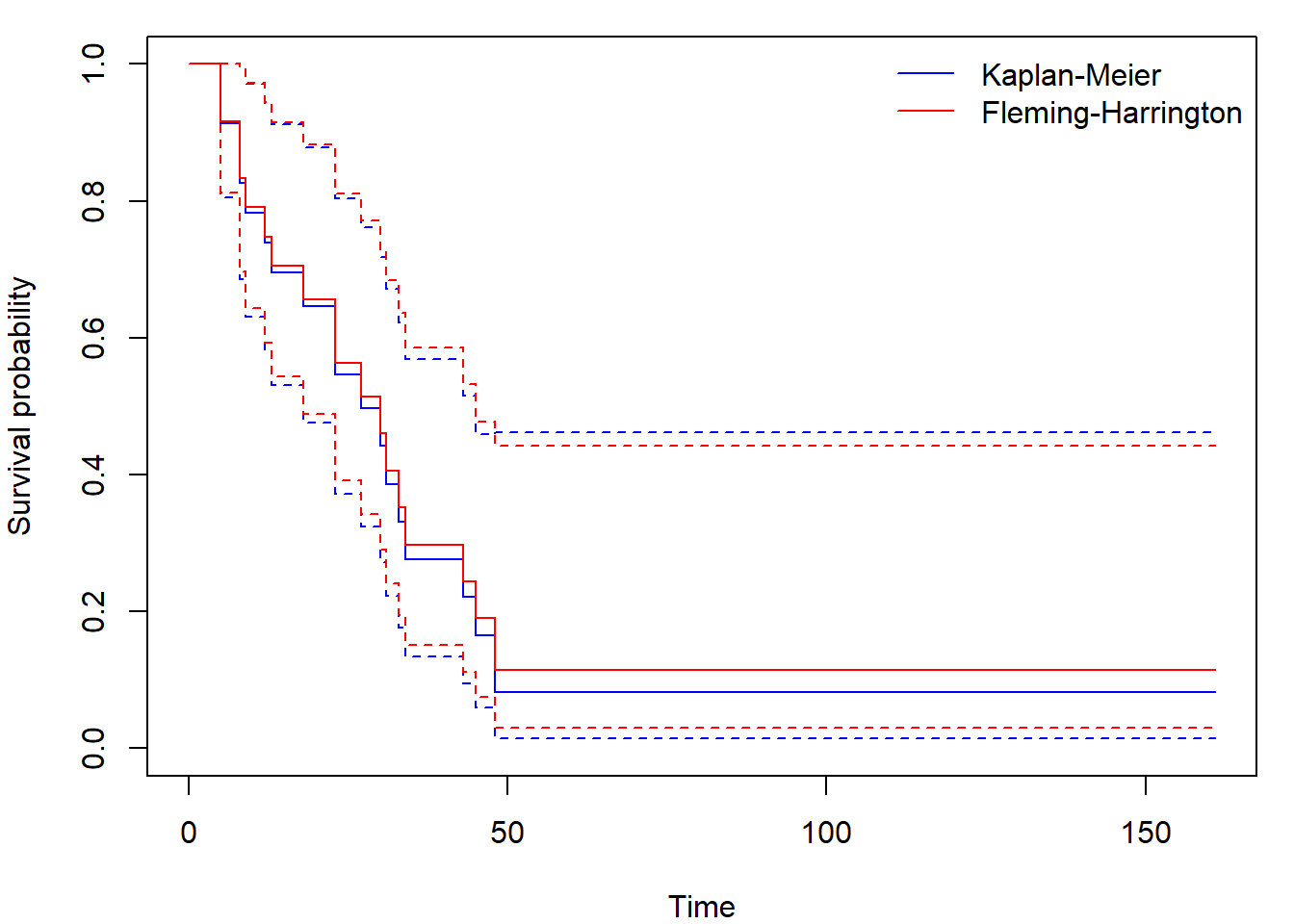
Sometimes you can come across figures with crosses at times where an
observation was censored (set mark.time = T, default
mark is +):
par(mar = c(4,4,1,1))
plot(fit_KM, mark.time = TRUE, conf.int = FALSE, col = "blue",
     xlab = "Time", ylab = "Survival probability")
legend("topright", "Kaplan-Meier",
       col = "blue", lty = 1, bty = "n")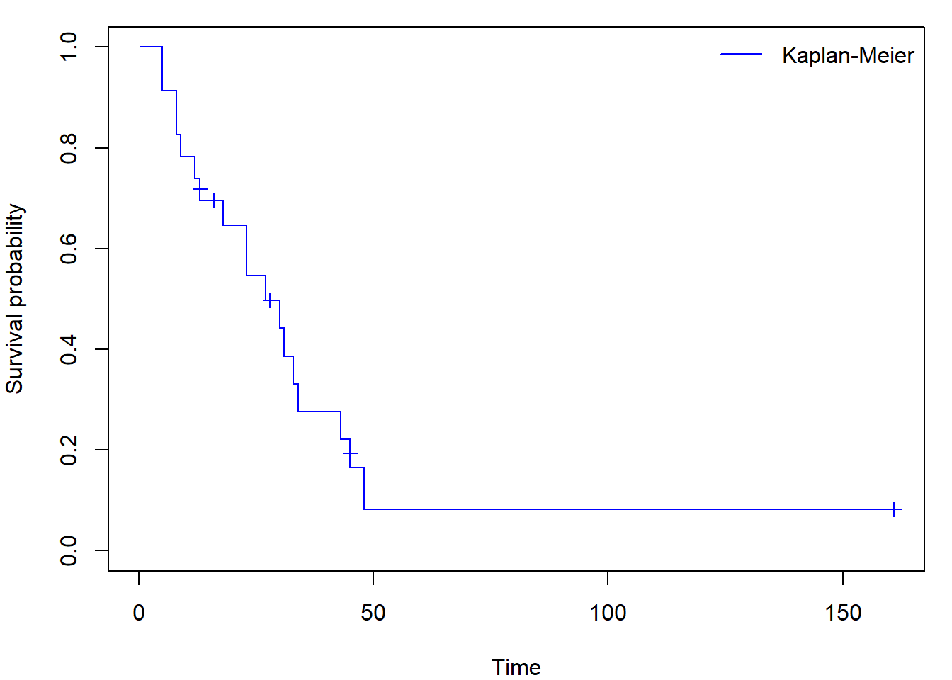
Using the formula notation, we can easily create and plot separate
curves for two distinct subgroups of observations (declared by factor
variable x within model formula instead of
1):
fit_gr <- survfit(Surv(time, status) ~ x, data = aml)
par(mar = c(4,4,1,1))
plot(fit_gr, xlab = "Time", ylab = "Survival probability", col = c("green","magenta"))
legend("topright", levels(aml$x), col = c("green","magenta"), lty = 1, bty = "n")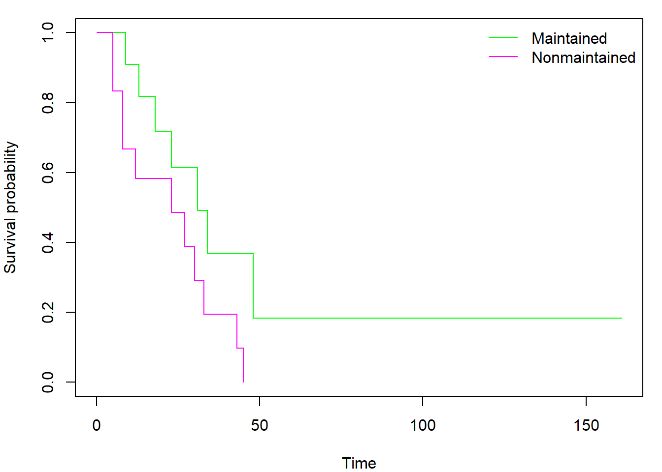
It is interesting to investigate the contents of the
survfit object by calling str(fit_KM). By
doing so, you may discover also the Nelson-Aalen estimator of cumulative
hazard function hidden in $cumhaz. Regardless of selected
type (kaplan or fleming)
$cumhaz always contains Nelson-Aalen estimator. If you need
cumulative hazard estimator derived from Kaplan-Meier estimator of
survival function you have to use the transformation \(\Lambda(t) = - \log \left( S(t) \right)\).
You can also easily plot the cumulative hazard function(s) by adding
fun = "cumhaz" into the plot command (see
help(plot.survfit) for other uses of fun
parameter):
par(mar = c(4,4,1,1))
plot(fit_gr, xlab = "Time", ylab = "Cumulative hazard function",
     col=c("green","magenta"), fun = "cumhaz")
legend("topright", levels(aml$x), col = c("green","magenta"), lty = 1, bty = "n")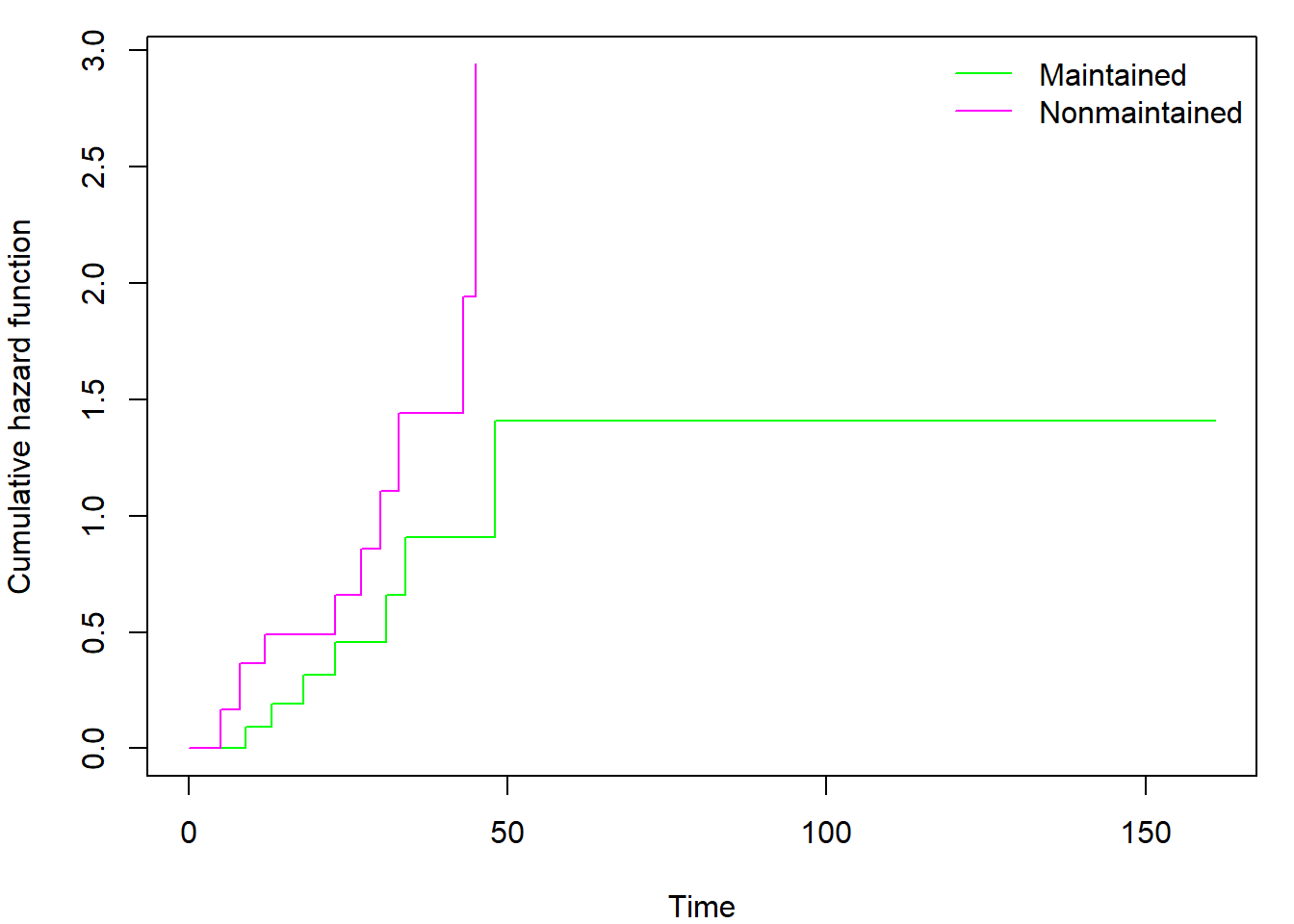
You can also use library(ggplot2) in cooperation with
library(survminer) to obtain nicer plots:
library(survminer)
library(ggplot2)
ggsurvplot(fit_gr, conf.int = TRUE, censor = TRUE,
           ggtheme = theme_minimal())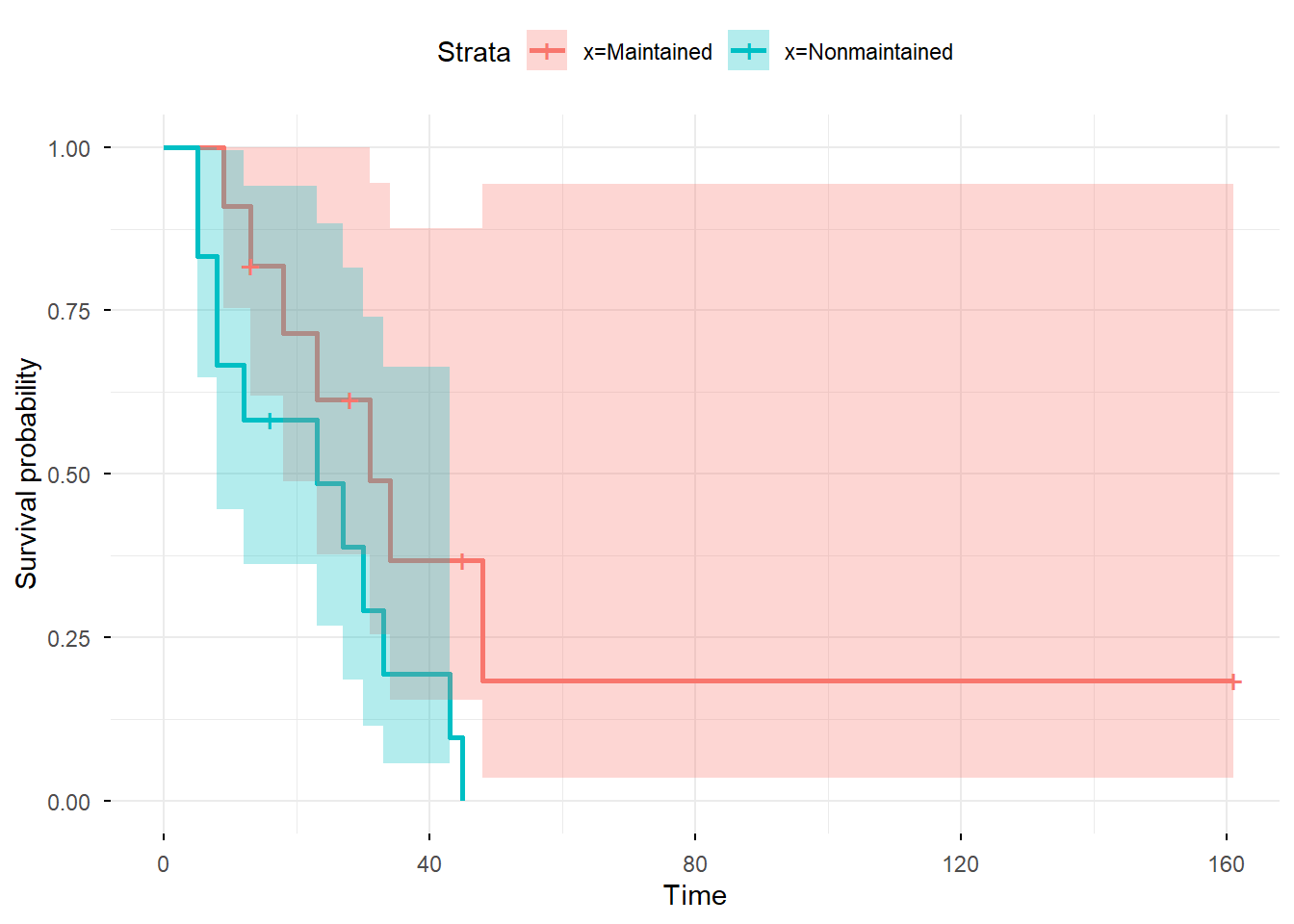
Calculate and plot the cumulative hazard estimator and both survival
function estimators for fans data using the function
survfit. Compare the results to those you obtained in Task
1. Include the code, output and comments in your report.
Advice: If not satisfied with the default plots of
plot.survfit, implement your own.
Simultaneous confidence bands
Asymptotic simultaneous \(100(1-\alpha)\)% Hall-Wellner confidence bands for \(S(t)\) over \(t\in[ 0,\tau]\) (for some pre-specified \(\tau\)) are \[ \biggl( \widehat{S}(t)\Bigl\{1-k_{1-\alpha}(\tau) %(\widehat{K}(\tau)) \bigl[1+\widehat{\sigma}(t)\bigr]/\sqrt{n}\Bigr\},\, \widehat{S}(t)\Bigl\{1+k_{1-\alpha}(\tau) %(\widehat{K}(\tau)) \bigl[1+\widehat{\sigma}(t)\bigr]/\sqrt{n}\Bigr\} \biggr), \] where \(\widehat{K}(t)=\widehat{\sigma}(t)/[1+\widehat{\sigma}(t)]\) and \(k_{1-\alpha}(t)\), \(t\in(0,1]\), satisfies the equation \[ \text{P}\bigl[\sup_{u\in [0,t]}|B(u)|>k_{1-\alpha}(t)\bigr]=\alpha, \] where \(B\) is the Brownian bridge.
There are variations of confidence intervals and confidence bands for
\(S(t)\) based on various
transformations (\(\log\), \(\log(-\log)\), \(\arcsin\), …), see parameter
conf.type. Formulae for these intervals can be derived by
the delta method.
The use of the delta-method: pointwise CI.
There are two different R libraries that can calculate Hall-Wellner simultaneous confidence bands.
1) library(km.ci)
This library includes a function called km.ci, which
requires a survfit object as the input and returns another
survfit object with recalculated lower and
upper components. The output can be processed by any
function that accepts survfit objects – e.g.,
plot, summary, lines.
library("km.ci")
fit <- survfit(Surv(time,status)~1, data=aml, conf.type="plain", conf.int=0.95)
out <- km.ci(fit, conf.level=0.95, tl=5, tu=48, method="hall-wellner")
par(mar = c(4,4,1,1))
plot(out, xlab = "Time", ylab = "Survival Probability")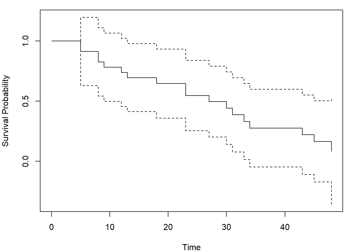
The arguments tl and tu are lower and upper
limits of the interval for which the bands are calculated. Not all
choises of these limits will lead to a useful result, so be careful and
try different inputs. Default values are set to the smallest and largest
event time (tl = min(aml$time[as.logical(aml$status)]) = 5,
tu = max(aml$time[as.logical(aml$status)]) = 48).
Other methods for calculating confidence intervals are
the following:
- pointwise:
peto,linear,log,loglog,rothman,grunkemeier, - simultaneous:
hall-werner,loghall,epband,logep.
See Details of km.ci function for explanation of these
abbreviations.
2) library(OIsurv)
This library includes a function called confBands, which
requires a survival object (just Surv) as the input and
returns a list of three vectors (time, lower,
upper). There is a method for plotting lines
from a confBands object, but no method for
plot!
Caution
The library OIsurv has been removed from CRAN. The last
version can still be installed from an archive, e.g. by the command
install.packages("http://www.karlin.mff.cuni.cz/~vavraj/nmst511/data/OIsurv_0.2.zip", repos =NULL)
## or from github if you use R-version 4.0.0 or higher
library("remotes")
install_github("cran/OIsurv")
Then one can obtain Hall-Wellner confidence bands as follows
library("OIsurv")
out <- confBands(Surv(aml$time,aml$status), confType="plain", confLevel=0.95, type="hall", tU=160)
par(mar = c(4,4,1,1))
plot(fit, xlab = "Time", ylab = "Survival probability", ylim = c(0,1))
lines(out, lty = 3, col = "blue")
legend("topright", c("Kaplan-Meier", "Pointwise confidence interval", "Hall-Werner confidence bands"),
       col = c("black", "black", "blue"), lty = c(1,2,3), bty = "n")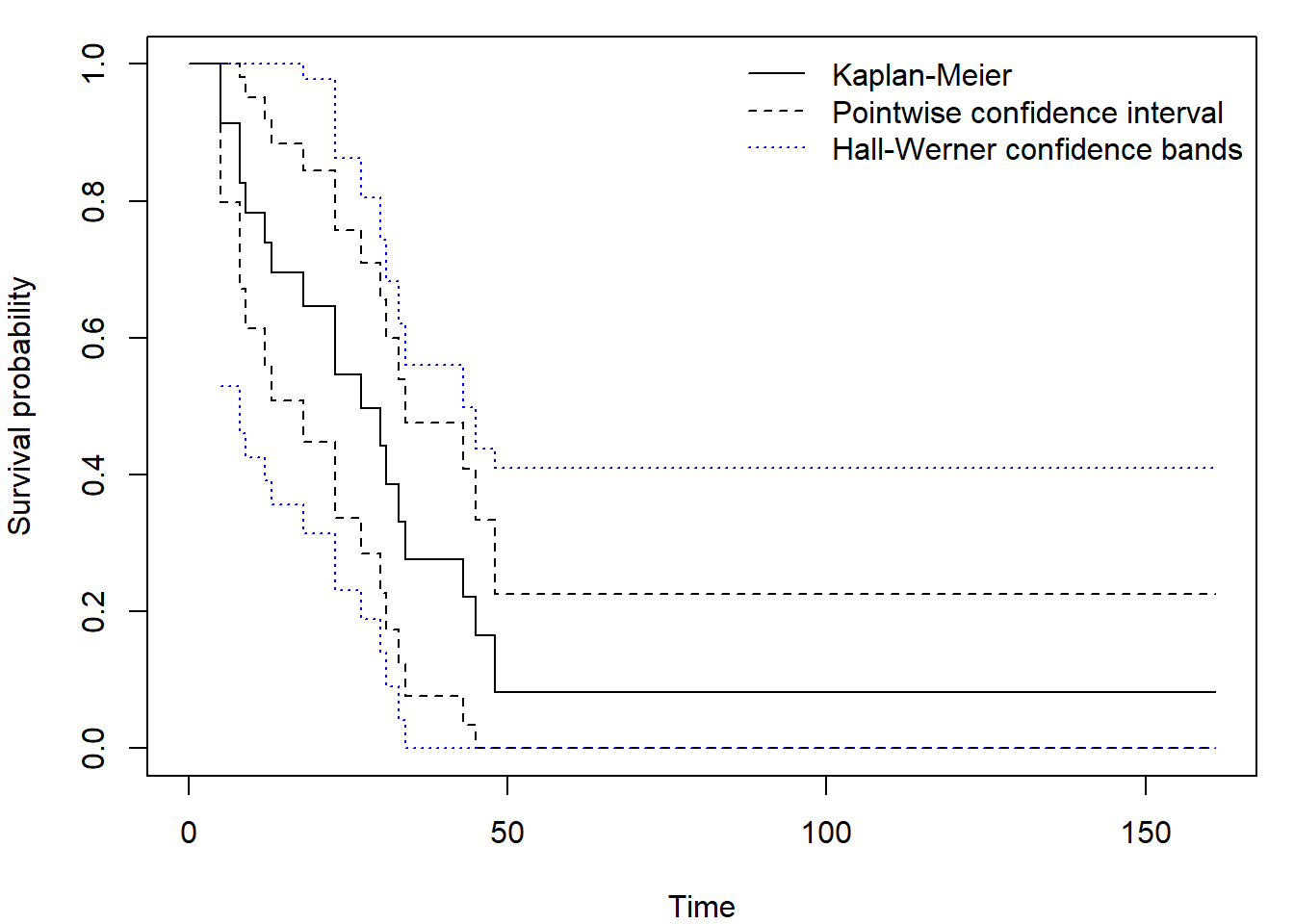
Again be careful when setting minimum tL and maximum
tU time value, the defaults are
tL = min(aml$time)= 5 = first observed or censored time,tU = max(aml$time)= 161 = last observed time.
Only confidence levels confLevel = c(0.9, 0.95, 0.99)
are accepted - default is 0.9!
Argument type differentiates between Equal precision
bands ("ep") and Hall-Werner ("hall" or just
"h"). You can also use different versions obtained by
application of Delta theorem:
confType = c("plain", "log-log", "asin-sqrt").

Generate \(n=50\) censored observations as follows. The survival distribution is Weibull with shape parameter \(\alpha=0.7\) and scale parameter \(1/\lambda=2\). Its expectation is \(\Gamma(1+1/\alpha)/\lambda=2\Gamma(17/7)\doteq 2.53\). The censoring distribution is exponential with rate \(\lambda=0.2\) (the expectation is \(1/\lambda=5\)), independent of survival.
Calculate and plot the Kaplan-Meier estimator of \(S(t)\) together with 95% pointwise confidence intervals and 95% Hall-Wellner confidence bands. Include the true survival function in the plot (use a different color). Include a legend explaining which curve is which and comment on the coverage.
Different format of the data
So far we have worked under the assumption that one row of the given data corresponds to one observation. However, often the data are already aggregated and different approach has to be taken.
Lifetable (actuarial) estimator
We do not have precise times of failure or censoring, only interval when it occurred. Given an interval we have total number of failures happening within the interval together with total number of units entering the interval (at risk of failure).
Notation:
- the \(j\)-th time interval is \([t_{j-1},t_j)\),
- \(c_j\) - the number of censorings in the \(j\)-th interval,
- \(d_j\) - the number of failures (deaths) in the \(j\)-th interval,
- \(r_j\) - the number of units entering the interval.
We could apply the K-M formula directly. However, it treats the
problem as though it were in discrete time, with events happening only
at endpoints of intervals. But the true events event times lie somewhere
within the preceding interval.
In fact, what we are trying to calculate here is the conditional
probability of dying within the interval, given survival to the
beginning of it.
We now make the assumption that the censoring process is such that the censored survival times occur uniformly throughout the \(j\)-th interval. So, we can assume that censorings occur on average halfway through the interval: \[ r_j'=r_j-c_j/2. \] I.e., average number of individuals who are at risk during this interval. This assumption yields the Actuarial Estimator. It is appropriate if censorings occur uniformly throughout the interval. This assumption is sometimes known as the actuarial assumption.
The event that an individual survives beyond \([t_{j-1},t_j)\) is equivalent to the event that an individual survives beyond \([t_{0},t_1)\) and … and that an individual survives beyond \([t_{j-2},t_{j-1})\) and that an individual survives beyond \([t_{j-1},t_j)\). Let us define the following quantities:
- \(P_j=P\{\mbox{an individual survives beyond }[t_{j-1},t_j)\}\),
- \(p_j=P\{\mbox{an individual survives beyond }[t_{j-1},t_j) |\mbox{ he survives beyond }[t_{j-2},t_{j-1})\}, \quad j>1\),
- \(p_1=P_1.\)
Then by chain rule, \(P_j=p_1 \cdot \; \cdots \; \cdot p_j.\) The conditional probability of an death in \([t_{j-1},t_j)\) given that the individual survives beyond \([t_{j-2},t_{j-1})\) is estimated by \(d_j/r_j'\). Thus, \(p_j\) is estimated by \[ \frac{r_j'-d_j}{r_j'}. \] So, the actuarial (lifetime) estimate of the survival function is \[ \widehat{S}(t)=\prod_{j=1}^{k-1}\frac{r_j'-d_j}{r_j'} \qquad \text{for } t_{k-1} \leq t < t_{k}. \]
Remarks:
- Because the intervals are defined as \([t_{j-1}, t_j)\), the first interval typically starts with \(t_0 = 0\).
- The implication in
Ris that \(\widehat{S}(t_0)=1\).
The form of the estimated survival function obtained using this method is sensitive to the choice of the intervals used in its construction. On the other hand, the lifetable estimate is particularly well suited to situations in which the actual death times are unknown, and only available information is the number of deaths and the number of censored observations which occur in a series of consecutive time intervals.
This heuristic is very similar to the used when dealing with interval censoring. However, it does not correspond to this case completely, as censoring times are not fully observed either. More on interval censoring and Turnbull estimator (generalization of KM estimator) can be found in Survival Analysis with Interval-Censored Data (2018) by Bogaerts, Komárek and Lesaffre.
Quantities estimated:
- Midpoint \(t_{mj}=(t_j+t_{j-1})/2\).
- Width \(b_j=t_j-t_{j-1}\).
- Conditional probability of dying \(\widehat{q}_j=d_j/r_j'\).
- Conditional probability of surviving \(\widehat{p}_j=1-\widehat{q}_j\).
- Cumulative probability of surviving at \(t_j\): \(\widehat{S}(t)=\prod_{l\leq j}\widehat{p}_l\).
- Hazard in the \(j\)-th interval \[ \widehat{\lambda}(t_{mj})=\frac{\widehat{q}_j}{b_j(1-\widehat{q}_j/2)} \] the number of deaths in the interval divided by the average number of survivors at the midpoint.
- Density at the midpoint of the \(j\)-th interval \[ \widehat{f}(t_{mj})=\frac{\widehat{S}(t_{j-1})\widehat{q}_j}{b_j}. \]
Constructing the lifetable:
In R function lifetab from
KMsurv package (KM stands for Klein and Moeschberger, not
Kaplan-Meier!) requires four elements:
library(KMsurv)
lifetab(tis,    #[K+1] a vector of end points of time intervals (including t_0)
        ninit,  #[1]   the number of subjects initially entering the study
        nlost,  #[K]   a vector of the number of individuals lost follow or withdrawn alive for whatever reason
        nevent) #[K]   a vector of the number of individuals who experienced the event
The output then contains:
nsubs- the number of subject entering the intervals who have not experienced the event.nlost- the number of individuals lost follow or withdrawn alive for whatever reason.nrisk- the estimated number of individuals at risk of experiencing the event.nevent- the number of individuals who experienced the event.surv- the estimated survival function at the start of the intervals.pdf- the estimated probability density function at the midpoint of the intervals.hazard- the estimated hazard rate at the midpoint of the intervals.se.surv- the estimated standard deviation of survival at the beginning of the intervals.se.pdf- the estimated standard deviation of the probability density function at the midpoint of the intervals.se.hazard- the estimated standard deviation of the hazard function at the midpoint of the intervals Therow.namesare the intervals.
Let us consider fans dataset with observations
grouped
tis <- seq(0, 120, by = 10)
fans$gtime <- cut(fans$time, breaks = tis)
fans$end_gtime <- as.numeric(fans$gtime) * 10 # end of intervals
tab <- table(fans$gtime, fans$fail)           # counts of censored and failed within time intervals

fitlt <- lifetab(tis = tis, ninit = dim(fans)[1], nlost = tab[,1], nevent = tab[,2])
fitlt
## nsubs nlost nrisk nevent surv pdf hazard se.surv se.pdf se.hazard
## 0-10 70 1 69.5 1 1.0000000 0.001438849 0.001449275 0.00000000 0.001428460 0.001449237
## 10-20 68 7 64.5 3 0.9856115 0.004584240 0.004761905 0.01428460 0.002585282 0.002748508
## 20-30 58 8 54.0 3 0.9397691 0.005220940 0.005714286 0.02921364 0.002933876 0.003297798
## 30-40 47 3 45.5 2 0.8875597 0.003901361 0.004494382 0.04024143 0.002703161 0.003177205
## 40-50 42 15 34.5 1 0.8485461 0.002459554 0.002941176 0.04698637 0.002427470 0.002940858
## 50-60 26 0 26.0 0 0.8239506 0.000000000 0.000000000 0.05166232 NaN NaN
## 60-70 26 7 22.5 1 0.8239506 0.003662003 0.004545455 0.05166232 0.003587056 0.004544280
## 70-80 18 3 16.5 0 0.7873305 0.000000000 0.000000000 0.06097909 NaN NaN
## 80-90 15 8 11.0 1 0.7873305 0.007157550 0.009523810 0.06097909 0.006846935 0.009513005
## 90-100 6 2 5.0 0 0.7157550 0.000000000 0.000000000 0.08792280 NaN NaN
## 100-110 4 3 2.5 0 0.7157550 0.000000000 0.000000000 0.08792280 NaN NaN
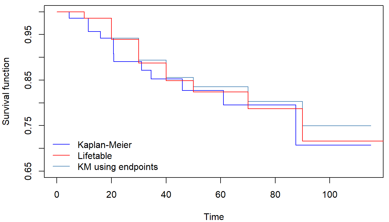
## 110-120 1 1 0.5 0 0.7157550 NA NA 0.08792280 NA NAfitKM_time <- survfit(Surv(time, fail) ~ 1, data = fans)
fitKM_end_gtime <- survfit(Surv(end_gtime, fail) ~ 1, data = fans)Actuarial estimate yields estimates much closer to the original Kaplan-Meier estimator (estimated with the exact known times) than Kaplan-Meier estimated with the times rounded up to the closest 10:
 This grouped data approach enables us to estimate the hazard functions
using formulae in the section above. The resulting estimate can be found
in
This grouped data approach enables us to estimate the hazard functions
using formulae in the section above. The resulting estimate can be found
in hazard output of lifetab function.
We will not dive deep into the theory, but there is also a method for
obtaining smoothed estimator of hazard function using
library(muhaz). Check that these methods provide similar
results:
library(muhaz)
haz <- muhaz(fans$time, fans$fail)

par(mfrow = c(1,1), mar = c(4,4,1,0.5))
plot(haz, col = "blue", xlab="Time", ylab= "Hazard function", ylim = c(0,0.01))
lines(tis, c(1, fitlt$hazard), col = "red", type = "S")
legend("top", c("Smoothed estimator", "Lifetable estimator"),
       col = c("blue", "red"), lty = 1, bty = "n", ncol = 2)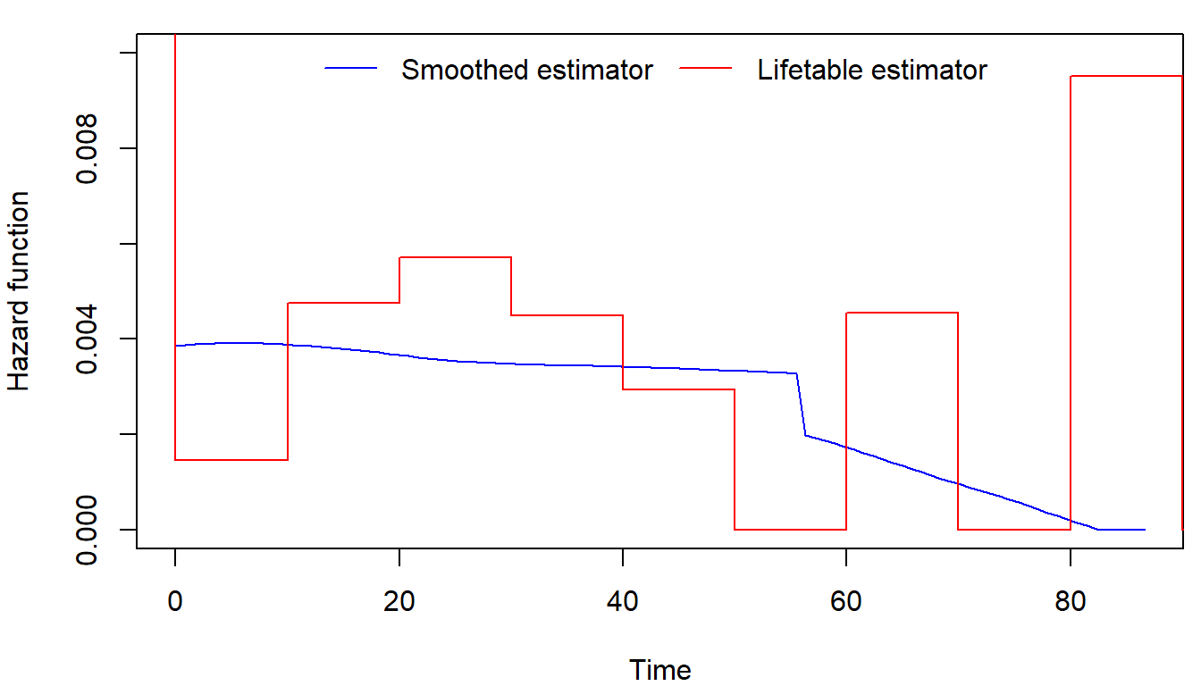
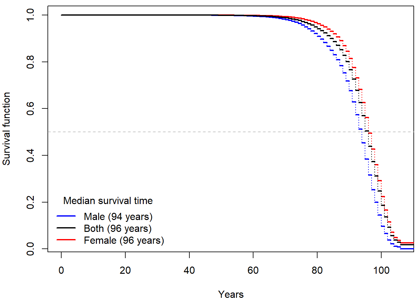
Mortality in the Czech Republic
Download dataset mort.RData. There are three
dataframes mort.m, mort.f and
mort containing mortality data from the Czech Republic in
the year 2021 for males, females and both genders combined. Each
dataframe has three columns:
iis an age group (going from the age \(i\) years to \(i+1\) years),Diis the number of deaths in the \(i\)-th age group in 2021,Yiis the number of people alive when they reached the age \(i\) (all at risk in \(i\)-th age group).
Think properly about the structure of this dataset. How does it differ from the formats above? What does belonging to a certain age group mean?
If we blindly use lifetab function
lt.f <- lifetab(tis = c(0,mort.f$i+1),              # age groups
                ninit = sum(mort.f$Yi),             # total number of women
                nlost = mort.f$Yi-mort.f$Di,        # number of survived in each age group
                nevent = mort.f$Di)                 # number of deaths in each age group
we obtain an absolute nonsense:
Each row can only be used to estimate the conditional probability of
surviving an age group. Thus, the resulting estimate of survival
function should be based on a product of 1 - Di/Yi.

Reproduce the plot above and compare your results to the official mortality tables created by ČSÚ: here for the males, here for the females. Can you recognize the columns in their table? Are their results comparable to yours?
If interested, examine the official guidelines (in Czech) of ČSÚ and see how the estimates could be further improved.
Include the (important) code, output and comments in your report.
- Deadline for report: Thursday 27 November 9:00
Historical evolution of survival probability in the state territory of the Czech Republic
Official estimates of the survival function given by ČSÚ in 1920-2021:
Show that the Nelson-Aalen estimator satisfies the equation \[ \sum_{i=1}^n \widehat{\Lambda}(X_i)=\sum_{i=1}^n \delta_i. \]
Show that under absence of censored data the Kaplan-Meier estimator becomes classical empirical estimator: \[ \widehat{S}(t) = \prod\limits_{\{j: t_j \leq t\}} \left[1 - \dfrac{\Delta\overline{N}(t_j)}{\overline{Y}(t_j)}\right] = \frac{1}{n}\sum \limits_{i=1}^n \mathbb{I}(X_i > t), \quad \forall t >0. \]