Testing equality of censored distributions
Jan Vávra
Exercise 3
Theory
The revision of the notation can be found in blackboard notes.
The two-sample problem in censored data analysis
We consider two independent censored samples of sizes \(n_1\) and \(n_2\), one sample with survival function \(S_1(t)\) and cumulative hazard \(\Lambda_1(t)\), the other sample with survival function \(S_2(t)\) and cumulative hazard \(\Lambda_2(t)\). The censoring distribution need not be the same in both groups.
Consider the hypothesis \[ \begin{aligned} \mathrm{H}_0: &\, S_1(t)=S_2(t) \quad \forall t>0, \\ \mathrm{H}_1: &\, S_1(t)\neq S_2(t) \quad \text{ for some } t>0, \end{aligned} \quad \Longleftrightarrow \quad \begin{aligned} \mathrm{H}_0: &\, \Lambda_1(t)=\Lambda_2(t) \quad \forall t>0, \\ \mathrm{H}_1: &\, \Lambda_1(t)\neq \Lambda_2(t) \quad \text{ for some } t>0. \end{aligned} \]
Weighted logrank statistics
The class of weighted logrank test statistics for testing \(H_0\) against \(H_1\) is \[ W_K=\int_0^\infty K(s)\,\mathrm{d}(\widehat{\Lambda}_1-\widehat{\Lambda}_2)(s), \] where \[ K(s)=\sqrt{\frac{n_1n_2}{n_1+n_2}} \frac{\overline{Y}_1(s)}{n_1}\, \frac{\overline{Y}_2(s)}{n_2}\,\frac{n_1+n_2}{\overline{Y}(s)}w(s) \] and \(w(s)\) is a weight function – it governs the power of the test against different alternatives.
\(w(s)=1\) is the logrank test. It is most powerful against proportional hazards alternatives, i.e., \(\lambda_1(t)=c\lambda_2(t)\) for some positive constant \(c\neq 1\).
\(w(s)=\overline{Y}(s)/(n+1)\) is the Gehan-Wilcoxon test which in the uncensored case is equivalent to two-sample Wilcoxon test. This test puts more weight on early differences in hazard functions than on differences that occur later.
\(w(s)=\widehat{S}(s-)\) is the Prentice-Wilcoxon test (also known as Peto-Prentice or Peto and Peto test). It is especially powerful against alternatives with strong early effects that weaken over time. Preferred compared to Gehan-Wilcoxon test.
\(w(s)=\left[\widehat{S}(s-)\right]^\rho\left[1-\widehat{S}(s-)\right]^\gamma\) is the \(G(\rho,\gamma)\) class of tests of Fleming-Harrington. The logrank test is a special case for \(\rho=\gamma=0\), the Prentice-Wilcoxon test is a special case for \(\rho=1,\ \gamma=0\). The \(G(0,1)\) test is especially powerful against alternatives with little initial difference in hazards that gets stronger over time.
Let \(\widehat\sigma^2_K\) be the estimated variance of \(W_K\) under \(H_0\), which is of the form \[ \widehat{\sigma}_K^2 = \int \limits_{0}^{\infty} \dfrac{K^2(s)}{\overline{Y}_1(s) \overline{Y}_2(s)} \left(1 - \dfrac{\Delta \overline{N}(s)-1}{\overline{Y}(s) - 1}\right) \,\mathrm{d} \overline{N}(s). \] It can be shown that, under \(H_0\), \[ \frac{W_K}{\widehat\sigma_K} \underset{n\to \infty}{\overset{\mathcal{D}}{\longrightarrow}} \mathsf{N}(0,1) \qquad\text{ and }\qquad \frac{W^2_K}{\widehat\sigma^2_K} \underset{n\to \infty}{\overset{\mathcal{D}}{\longrightarrow}} \chi^2_1. \]
Calculation of weighted logrank statistics
Let \(t_1<t_2<\cdots<t_d\) be the ordered distinct failure times in both samples. The weighted logrank test statistic (without the normalizing constant depending on \(n_1\) and \(n_2\)) can be written as \[ \sum_{j=1}^d \biggl(\Delta\overline{N}_1(t_j)-\Delta\overline{N}(t_j) \frac{\overline{Y_1}(t_j)}{\overline{Y}(t_j)}\biggr) w(t_j). \] The variance estimator \(\widehat{\sigma}_K^2\) (again without the normalizing constant depending on \(n_1\) and \(n_2\)) can be calculated using the following formula \[ \sum \limits_{j = 1}^d \Delta N(t_j) \cdot \dfrac{\overline{Y}_1(t_j) \overline{Y}_2(t_j)}{\left(\overline{Y}(t_j)\right)^2} \cdot \dfrac{\overline{Y}(t_j) - \Delta N(t_j)}{\overline{Y}(t_j) - 1} \cdot \left(w(t_j)\right)^2. \]
Download the dataset km_all.RData.
The dataframe inside is called all. It includes 101
observations and three variables. The observations are acute lymphatic
leukemia [ALL] patients who had undergone bone marrow transplant. The
variable time contains time (in months) since
transplantation to either death/relapse or end of follow up, whichever
occured first. The outcome of interest is time to death or
relapse of ALL (relapse-free survival). The variable
delta includes the event indicator (1 = death or relapse, 0
= censoring). The variable type distinguishes two different
types of transplant (1 = allogeneic, 2 = autologous).
Using ordinary R functions (not the survival library),
calculate and print the following table:
| \(j\) | \(t_j\) | \(d_{1j}\) | \(d_{j}\) | \(y_{1j}\) | \(y_j\) | \(e_j=d_j\frac{y_{1j}}{y_j}\) | \(d_{1j}-e_j\) | \(v_j=d_j\dfrac{y_{1j} (y_j-y_{1j}) (y_j-d_j)}{y_j^2 (y_j - 1)}\) |
|---|---|---|---|---|---|---|---|---|
| 1 | … | … | … | … | … | … | … | … |
| … | … | … | … | … | … | … | … | … |
| d | … | … | … | … | … | … | … | … |
where \(j\) is the order of the failures, \(t_j\) is the ordered failure time, \(d_{1j}=\Delta\overline{N}_1(t_j)\), \(d_j=\Delta\overline{N}(t_j)\), \(y_{1j}=\overline{Y}_1(t_j)\), \(y_j=\overline{Y}(t_j)\).
Use these values to perform logrank test on your own.
BONUS: Try to implement \(G(\rho,\gamma)\) test, remember, you need left-continuous version of Kaplan-Meier estimator of survival function.
Implementation in R
The function survdiff in the library
survival can calculate \(G(\rho,0)\) statistics. The default is
\(\rho=0\), the logrank test. Output is
a list with:
$chisq- test statistic in the squared form \(W_K^2/\widehat{\sigma}_K^2\),$var[1,1]- variance estimator \(\widehat{\sigma}_K^2\),$pvalue- the p-value computed bypchisq(...$chisq, df=1, lower.tail = F),$obs[1]- is the first sum \(\sum\limits_{j=1}^d \Delta \overline{N}_1(t_j) w(t_j)\) corresponding to weighted observed failures in sample 1,$exp[1]- is the second sum \(\sum\limits_{j=1}^d \Delta \overline{N}(t_j) \frac{\overline{Y}_1(t_j)}{\overline{Y}(t_j)} w(t_j)\) corresponding to weighted expected failures under the null (same survival distributions) in sample 1.
library(survival)
survdiff(Surv(time, delta) ~ type, data = all)
survdiff(Surv(time, delta) ~ type, data = all, rho=2)
## Call:
## survdiff(formula = Surv(time, delta) ~ type, data = all)
##
## N Observed Expected (O-E)^2/E (O-E)^2/V
## type=1 50 22 24.2 0.195 0.382
## type=2 51 28 25.8 0.182 0.382
##
## Chisq= 0.4 on 1 degrees of freedom, p= 0.5The function FHtestrcc in the library
FHtest can calculate \(G(\rho,\gamma)\) statistics for non-zero
\(\gamma\). The default is \(\rho=0,\ \gamma=0\), the logrank test. The
parameter \(\gamma\) is entered as the
argument lambda. For the proper choice of \(\rho\) and \(\gamma\) read Details of
help(FHtestrcc). Output is a list with:
$statistic- test statistic in the form \(W_K/\widehat{\sigma}_K\),$var- variance estimator \(\widehat{\sigma}_K^2\),$pvalue- p-value of the test associated with the selected alternative hypothesis (parameteralternative),- …
library(FHtest)
FHtestrcc(Surv(time, delta) ~ type, data = all)
FHtestrcc(Surv(time, delta) ~ type, data = all, rho=0.5, lambda=2)
##
## Two-sample test for right-censored data
##
## Parameters: rho=0.5, lambda=2
## Distribution: counting process approach
##
## Data: Surv(time, delta) by type
##
## N Observed Expected O-E (O-E)^2/E (O-E)^2/V
## type=1 50 0.961 1.69 -0.732 0.316 5.63
## type=2 51 2.369 1.64 0.732 0.327 5.63
##
## Statistic Z= 2.4, p-value= 0.0176
## Alternative hypothesis: survival functions not equalCaution
The library FHtest requires library Icens
which has been removed from R and cannot be installed by standard
methods. It is available from the Bioconductor
repository. It can be downloaded manually and installed by a command
such as:
install.packages("http://www.karlin.mff.cuni.cz/~vavraj/nmst511/data/Icens_1.80.0.tar.gz", repos=NULL)
# or if you have troubles with R version, try
library("remotes")
install_github("cran/Icens")survdiff and FHtestrcc output)
Compare your calculation of logrank test with the output of the
functions survdiff and FHtestrcc in the case
of dataset all.
In the all data, investigate the difference in survival
and hazard functions according to the type of transplant (1 =
allogeneic, 2 = autologous). Remember that the outcome is relapse-free
survival.
Calculate and plot estimated survival functions by the type of transplant. Distinguish the groups by color. Add a legend.
Calculate and plot Nelson-Aalen estimators of cumulative hazard functions by the type of transplant. Distinguish the groups by color. Add a legend.
Calculate and plot smoothed hazard functions by the type of transplant. Distinguish the groups by color. Add a legend.
Perform logrank, Prentice-Wilcoxon and \(G(0,1)\) tests using functions
survdifforFHtestrcc. Interpret the results. Which test is more suitable in this case?
Hint for obtaining smoothed hazard functions:
library(muhaz)
haz = muhaz(all$time, all$delta)
plot(haz, col = "black", lwd = 2)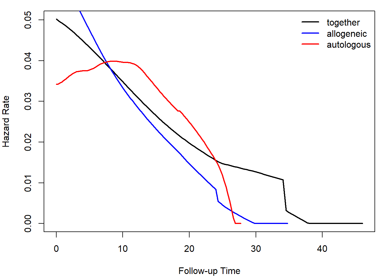
The choice of two-sample test statistic
To succesfully complete the following task use the following shiny app.
Fill the following table with the symbols:
- 1 = super choice,
- 2 = good choice,
- 3 = inappropriate/bad choice,
- ? = no idea.
This symbol will represent your opinion on the choice of this particular two-sample statistic in the case of violation null hypothesis described by the plot of hazard functions.
Using the shiny app find at least one example (distributions of survival times \(T_1\), \(T_2\) and their censoring distributions) where logrank is inappropriate (low power under evident H0 violation) while some other weight function rejects obvious violation of null hypothesis.
| Statistic | Weight function | \(G(\rho, \gamma)\) |  |
 |
 |
 |
 |
 |
|
|---|---|---|---|---|---|---|---|---|---|
| Logrank (Mantel) | \(1\) | \(G(0,0)\) | |||||||
| Prentice-Wilcoxon | \(\widehat{S}(t-)\) | \(G(1,0)\) | |||||||
| — | \(\left[1-\widehat{S}(t-)\right]\) | \(G(0, 1)\) | |||||||
| Fleming-Harrington | \(\rho = \gamma = 1\) | \(G(1, 1)\) |
The rest of this exercise is focused on real data analyses with different hazard shapes.
Compare survival distributions between the two groups of interest in the following datasets. Conduct the analysis according to the same steps as in Task 2.
Calculate and plot survival function.
Calculate and plot Nelson-Aalen estimators of cumulative hazard function.
Plot smoothed hazard functions.
Perform logrank, Prentice-Wilcoxon, \(G(0,1)\) or some particular \(G(\rho,\gamma)\) tests using functions
survdifforFHtestrcc. Interpret the results. Discuss the choice of weight function with respect to the power of the resulting test.
Try to avoid repeating the same code in your solution over and over.
Activate the dataset veteran by calling
data(veteran). It includes 137 observations and eight
variables. The observations are lung cancer patients. The variable
time contains survival time (in days) since the start of
treatment. The variable status includes the event indicator
(1 = death, 0 = censoring). The variable trt distinguishes
two different treatments (1 = standard, 2 = experimental). The treatment
was randomly assigned to the patients.
Compare survival distributions between standard and experimental treatments.
Compare survival distributions between patients with Karnofsky scores up to 60 and over 60 (regardless of treatment assignment). These scores are stored in variable
karno.
You should also be able to perform some simulation study on your own:
Generate \(n_1=100\) censored observations from the Weibull distribution with shape parameter \(\alpha=0.7\) and scale parameter \(1/\lambda=2\). Its expectation is \(\Gamma(1+1/\alpha)/\lambda=2\Gamma(17/7)\doteq 2.53\).
Generate another sample of \(n_2=100\) censored observations from the exponential distribution with the same mean.
Let the censoring distribution in both samples be exponential with the rate \(\lambda=0.2\) (the expectation is \(1/\lambda=5\)), independent of survival. Put both samples in a single dataframe, introducing a variable distinguishing which sample each observation comes from.
Compare survival distributions between the two groups using the generated data. Conduct the analysis according to the steps 1–4 and display the true survival and hazard functions in the plots generated at steps 1–3 of the analysis.
- Deadline Tasks 1-6 : Thursday 18 December 9:00